Energy Use and GHG Emissions

Methods 5.0

Cradle-to-gate energy use and GHG emissions associated with the production of a crop.

The agricultural sector represents approximately 10% of the total greenhouse gas (GHG) emissions in the United States (USEPA 2023b). Quantifying GHG emissions at the field level enables stakeholders in the agriculture value chain to identify key sources of emissions, estimate the impact of alternative production scenarios, set sustainability goals, and report outcomes.

The methods behind the Field to Market [Energy Use] and [GHG Emissions] sustainability indicators are connected because some GHG emissions come from farming activities that consume energy like irrigation pumping or post-harvest drying. Other GHG emissions come from sources like upstream fertilizer production or methane or nitrous oxide released from soils. Fieldprint Platform v5 estimates energy use and GHG emissions using impact factors, Tier 1 and Tier 2 approaches, and process-based models, which are considered a Tier 3 approach by IPCC (IPCC 2019).

GHG emission quantification for agricultural production has advanced in rigor and standardization over the past fifteen years. The Fieldprint Platform v5 aligns with life cycle analysis (LCA) principles and major standards by updating system boundaries, impact factors and reference data, and revising and adding sources of GHG emissions.

Energy Use

The Energy Use calculations estimate the cumulative energy demand (CED) associated with producing a given crop, following a cradle-to-processing-gate system boundary. The CED accounts for the primary energy from fossil and non-fossil sources used throughout the life cycle, including upstream supply chains. In the Fieldprint Platform, Energy Use can be expressed as the sum of three components:

\[ Energy~ Use = E_{upstream} + E_{mechanical} + E_{post-harvest} \]

• Upstream: energy associated with electricity generation and distribution, transportation of agricultural inputs, and production of fuels, fertilizers, pesticides, and seed.
• Mechanical: energy associated with mobile and stationary machinery on-farm, such as tractors, combines, and irrigation pumps.
• Post-harvest: energy associated with mobile and stationary machinery outside the field or farm, such as crop transportation and drying.

The activities listed below consume energy and have associated GHG emissions. Click the links to learn more about these methods used in the Fieldprint Calculator.

GHG Emissions

The activities listed above use energy and have associated GHG emissions. Those emissions along with other sources and sinks for GHGs combine into the Field to Market GHG Emissions Indicator.

\[ GHG~ Emissions = GHG_{upstream} + GHG_{mechanical} + GHG_{non-mechanical} + GHG_{post-harvest} \]
where

• Upstream = emissions associated with electricity generation and distribution, transportation of agricultural inputs, and production of fuels, fertilizers, pesticides, and seed.
• Mechanical = emissions associated with mobile and stationary machinery on-farm.
• Non-mechanical = emissions associated with field-level CH₄ flux from non-flooded soils, CO₂ from carbonate lime applications to soils, CO₂ from urea fertilizer applications, non-CO₂ emissions from biomass burning, direct land use change emissions, soil N₂O, CH₄ emissions from flooded rice cultivation, and CO₂ from soil carbon stock changes.
• Post-harvest = emissions associated with mobile and stationary machinery outside the field or farm.

The GHG Emissions Indicator estimates the mass of gases in flux in the production of a given crop. The estimated gases are converted to Global Warming Potential (GWP) using 100-yr time horizon factors from the Intergovernmental Panel on Climate Change Sixth Assessment Report¹ (AR6) (Pier et al. 2021).

The methods for estimating GHGs from separate sources (or sinks) are listed below. Click the links to learn more.

Supplemental

Life Cycle Analysis

ImportantWhat is life cycle analysis (LCA)?

From ISO (2006) :

LCA is the compilation and evaluation of the inputs and outputs and the potential environmental impacts of a product system throughout its life cycle.

What is the use of LCA?

From Sieverding et al. (2020) :

Life cycle analysis is used to quantify the environmental performance of products, processes, or services, and is increasingly being used as a basis to inform purchasers along the supply chain, including the end users (Fava, Baer, and Cooper 2011).

The Fieldprint Platform is designed to produce an attributional, streamlined life cycle analysis of a given crop. Attributional LCAs are common in agriculture (Sieverding et al. 2020); the analysis is detailed and process-specific, which enables growers and organizations in the agricultural value chain to evaluate the environmental outcomes of business-as-usual practices, compare them with potential improvement scenarios, and find ways to incentivize practices for which there is evidence of a reduced environmental impact.

Streamlined LCA, as opposed to a traditional or full LCA, is a resource-efficient method to identify key contributors to GHG emissions, among other impacts (Pelton 2018; Verghese, Horne, and Carre 2010). Streamlined LCAs focus on limited impact categories and reduce the barriers to conducting assessments of the environmental impact of crop production (Pelton 2018). Agriculture is one of many industries utilizing streamlined LCA to detect the highest contributors of GHG emissions and other environmental impacts. The literature contains many examples of streamlined LCA from the automotive (Arena, Azzone, and Conte 2013), packaging (Verghese, Horne, and Carre 2010), solid waste management (Y. Wang, Levis, and Barlaz 2021), and construction (Heidari et al. 2019) industries.

The simplification of LCA could result in too many shortcuts and assumptions that jeopardize their accuracy and utility (Verghese, Horne, and Carre 2010; Hunt et al. 1998). The Fieldprint Platform’s streamlined LCA model aims to achieve an acceptable balance between the practicality and completeness of the analysis

Functional Unit

ImportantWhat is a functional unit?

From Sieverding et al. (2020):

• The unit for products or services at which LCA results are presented.
• The selection of functional units used in LCAs typically is closely related to the evaluation’s goals and frequently is expressed as a unit of area (e.g., hectare or acre) or mass (e.g., kg or bushel of grain, kg or lb of meat) for food-related LCAs.

In other words, the functional unit acts as the denominator for a given metric or impact category. For example, the GHG emissions associated with the production of peanuts as kg CO₂e / kg peanuts.

In version 5, the functional unit for [Energy Use] and [GHG Emissions] will be 1 kg of crop production output at standard moisture for all crops. In USCS units, the functional unit stays the same at 1 unit of crop production output at standard moisture (bushel, cwt, ton, and lb, depending on the crop). Crop production output is determined on the basis of yield for a given planted area.

For the Soil Carbon indicator, the functional unit is 1 hectare for SI units and 1 acre for USCS units.

System Boundary

ImportantWhat is a system boundary?

The system boundary is a definition of what is included or excluded from the analysis (Czyrnek-Delêtre, Smyth, and Murphy 2017).

For [Energy Use] and [GHG Emissions], the proposed system boundary will be cradle-to-processing-gate, which includes post-harvest activities such transportation from the field to the dryer, storage, or processing gate, and the crop drying activity. Cradle refers to the production of agricultural inputs and crop production (Bandekar et al. 2022), while processing gate refers to the inlet or the beginning of the processing of crop production output, such as cleaning, sorting, crushing, etc. The revised system boundary will include cover cropping activities and their upstream and on-farm impact. The time accounting will use a crop interval approach.

The system boundary for the Soil Carbon metric is similar, with the notable feature of time accounting based on a calendar year rather than crop interval.

The system boundary and disaggregation within the system were adapted from a framework described by Richards (2018), and is visualized below:

System boundary for the Fieldprint Platform Version 5.

Allocation

For all crops except one, the burden of materials, resources, and emissions is allocated to the harvested crops. No burden is assigned to the crop residue, byproducts, or co-products. The exception is cotton, for which members in the cotton industry requested an 83% economic allocation to the cotton lint vs. the seed.

Tiers

ImportantWhat are Tier 1, 2, and 3 approaches?

From the overview of IPCC (2019) :

• Tier 1 represents the simplest methods, using default equations and emission factors provided in the IPCC guidance.
• Tier 2 uses default methods, but emission factors that are specific to different regions.
• Tier 3 uses country‐specific estimation methods, such as a process‐based model.

GHG emission quantification approaches include multiple levels or tiers of complexity and accuracy, based on the best available data and methods.

The GHG emission methods published by Hanson et al. (2024) take a slightly modified approach from IPCC tiers, calling them instead Basic Estimation Equation, Inference, Modified IPCC or Empirical Model, and Processed‐Based Model. They are described as follows:

• Basic estimation equations use default equations and emission factors, such as IPCC Tier 1 methods.

• Inference uses geography‐, crop‐, livestock‐, technology‐, or practice‐specific emission factors to approximate emissions/removal factors. This approach is similar to an IPCC Tier 2 method and is more accurate, more complex, and requires more data inputs than the basic estimation.

• Modified IPCC/empirical and/or process‐based modeling, comparable to IPCC Tier 2 or IPCC Tier 3 methods. These methods are the most demanding in terms of complexity and data requirements and produce the most accurate estimates.

Impact Factors

Note: This section was authored by Rylie Pelton, Ph.D.²

To ensure the Fieldprint Platform comprehensively calculates GHG emissions and energy demand from a life cycle perspective, covering emissions from cradle-to-processing-gate as well as on-farm use, several modifications and additions have been made to the emission factors for key farm inputs, including electricity, fuels, fertilizers, inoculants, and pesticides. While many emission factors are available in commercial LCA databases, licensing constraints prevent their direct integration into the Fieldprint Platform, given Field to Market’s commitment to transparency. As a result, the methodology primarily relies on publicly available datasets and peer-reviewed literature to construct impact factors for energy demand and GHG emissions.

GHG emissions will be estimated using carbon dioxide equivalents (CO₂e) based on Global Warming Potential (GWP) values from the IPCC 6th Assessment Report (AR6), which incorporates the latest advancements in climate science (IPCC 2023). These factors include 100-year GWP values for methane (CH₄) (29.8) and nitrous oxide (N₂O) (273), with biogenic methane (CH₄) (27) explicitly categorized. GHG emissions are delineated by individual gas type to allow for flexibility in applying alternative GWP characterization factors (e.g. AR5 or AR4) to facilitate benchmarking and comparative analyses.

The Energy Use metric in the Fieldprint Platform, which previously represented only the energy consumed on the farm, has now been expanded to cumulative energy demand (CED), a life cycle-based metric that accounts for primary gross energy inputs, including both fossil and non-fossil (e.g., solar, wind, nuclear) energy. This metric captures not only direct combustion energy but also the energy required for extraction, refining, and production of energy carriers used throughout the agricultural supply chain for energy and materials.

These updates effectively expand the system boundaries within the Fieldprint Platform to a full cradle-to-gate life cycle assessment for both CED and GWP. The updates encompass a broader range of inputs, including inoculants, fertilizers and micronutrient fertilizers, pesticides, and fuel use applications, to better capture the diverse practices used on farms. Additionally, by delineating emissions by specific greenhouse gas types and separating direct from upstream contributions, these updated estimates offer enhanced flexibility for benchmarking and greater transparency for stakeholders. The following sections outline the data sources and methods used to update the emission factors for each input category.

Electricity

Electricity emissions are calculated based on regional grid mixes to ensure increased accuracy in estimating GHG emissions from electricity use in agricultural production. Given the variability in energy generation sources across the U.S., electricity emission factors are estimated for 27 U.S. subregions, using data from the EPA’s eGRID database for the latest reporting year (O. USEPA 2023). This approach ensures the electricity related emissions reflect regional energy supply characteristics, including the proportion of fossil fuel, nuclear, hydroelectric, wind and solar generation in each subregion.

To determine total electricity-related emissions, both direct emissions from fossil fuel combustion in power plants, and upstream emissions from fuel extraction, refining, processing and distribution, are considered. Direct emissions are sourced from EPA eGRID data, which provides CO₂, CH₄, and N₂O emissions per MWh of electricity generated (USEPA 2023a). Since electricity generation involves significant energy losses during fuel conversion, emission factors account for power plant efficiency and fuel-specific combustion characteristics.

In addition to direct emissions, upstream emissions associated with energy production and delivery are incorporated to capture the full life cycle impact of electricity use. These include GHG emissions from fuel extraction, refining, and distribution of each energy source (LEIF 2025; National Renewable Energy Laboratory 2012). Additionally, electricity losses occur during transmission and distribution (T&D), reducing the net electricity available for energy use applications. Regional T&D loss factors area applied to adjust the emission factors accordingly, ensuring that emissions reflect actual electricity delivered to agricultural operations (USEPA 2025).

Fuels

Fuel emission factors encompass both combustion emissions and upstream emissions associated with fuel extraction, distribution, and refining. Combustion emissions are derived from the EPA Emission Factor Hub, which provides estimates of CO₂, CH₄, and N₂O emissions per unit of fuel combusted (USEPA 2023a). Since fuel-related emissions vary depending on whether the fuel is used in stationary combustion equipment (e.g. grain dryers) or mobile applications (e.g. tractors, off-road agricultural machinery and trucks, and on-road trucks), separate emission factors are applied for each category.

For stationary combustion, the EPA emission factors are provided per unit of higher heating value (HHV). However, most agricultural and transportation applications do not utilize the latent heat from fuel combustion, as vapor recondensing technologies are uncommon in these sectors, and therefore energy usage for agricultural and transportation operations are measured in lower heating value (LHV) energy units. To align the emission estimates with agricultural energy use practices, we convert HHV based emission factors into LHV-based factors using standard conversion factors for each fuel type (Tools 2024; USEPA 2023a). For mobile combustion, fuel-specific emission factors are applied based on mode-specific data for off-road trucks and machinery, on-road trucks, and other agricultural vehicles. These values reflect variations in engine efficiencies, combustion conditions, and regulatory emission controls across different fuel applications (USEPA 2023a).

In addition to combustion emissions, upstream emissions from fuel production are incorporated into the analysis to account for cradle-to-processing-gate emissions, including from fuel extraction, transport, refining, and processing. The GREET 2023 model is used to estimate GHG emissions per MJ (LHV) of fuel throughput, ensuring all stages of fuel production are properly captured (M. Wang et al. 2023). Furthermore, GREET provides estimated cumulative energy demand (CED) per unit of fuel throughput. For example, for every MJ of diesel combusted, the CED is 1.12 MJ, reflecting both direct combustion energy and the additional energy required for extraction, refining, and distribution. For renewable soy biodiesel fuels, CED and GWP capture impacts from soybean cultivation, crushing, and biodiesel processing (M. Wang et al. 2023).

Fertilizers

Cradle-to-processing-gate emissions from fertilizer are primarily based on the Argonne National Laboratory (ANL) GREET Feedstock Carbon Intensity Calculator (FD-CIC) (Liu et al. 2023). This tool quantifies emissions from major fertilizer types, including ammonia, urea ammonium nitrate, urea ammonium nitrate, and others. The FD-CIC tool details the material and energy inputs required for fertilizer production, incorporating emissions from direct fuel combustion, chemical process emissions, and upstream material extraction and intermediary processing (Liu et al. 2023). To supplement the FD-CIC data for fertilizer types not included in the tool, additional emission factors are incorporated from other LCA databases (e.g. USLCI) and peer-reviewed literature (Gaidajis and Kakanis 2020; LEIF 2025; Fertilizers Europe 2024). Table 1 shows the primary sources of information for the various fertilizer options. CED for each material and energy input is based on National Renewable Energy Laboratory (2012) and LEIF (2025). The top eight fertilizers include both conventional and green production pathways, where ammonia is produced via electrolysis using hydrogen and nitrogen, resulting in fertilizers with lower carbon intensities compared to conventional production.

Table 1: Sources of impact factors for fertilizer options

Fertilizer	Primary Sources
Ammonia	Liu et al. (2023)
Urea	Liu et al. (2023)
Ammonium nitrate	Liu et al. (2023)
Ammonium sulfate	Liu et al. (2023)
Urea ammonium nitrate	Liu et al. (2023)
Calcium ammonium nitrate	Fertilizers Europe (2024); Liu et al. (2023)
Monoammonium phosphate	Liu et al. (2023)
Diammonium phosphate	Liu et al. (2023)
Potassium nitrate	Liu et al. (2023); LEIF (2025)
Sulfur	Liu et al. (2023); National Renewable Energy Laboratory (2012)
Lime	Liu et al. (2023)
Muriate of potash	Liu et al. (2023)
Boric acid	Liu et al. (2023); LEIF (2025); Gaidajis and Kakanis (2020)
Zinc sulfate	Liu et al. (2023); LEIF (2025); Gaidajis and Kakanis (2020)
Manganese oxide	Liu et al. (2023); LEIF (2025); National Renewable Energy Laboratory (2012)

The FD-CIC tool provides a breakdown of process emissions, representing the direct emissions associated with fuel combustion during production, as well as emissions released during chemical transformations. For instance, during the production of ammonia-based fertilizers, ammonia leakage contributes to indirect nitrous oxide emissions. The FD-CIC tool specifies total GHG emissions per unit of fertilizer production, differentiating between direct CO₂ emissions and total GHG emissions. The remaining GHG emissions (CH₄ and N₂O) are allocated based on the proportion of upstream emissions attributed to each gas type (Liu et al. 2023). We combine the material and energy input inventories for each of the fertilizer types with the cradle-to-gate emission factors included in the FD-CIC tool, including, for example, natural gas, diesel, nitric acid, and electricity.

The cumulative energy demand (CED) of fertilizer production is estimated by integrating energy input requirements for each production process with cradle-to-processing-gate CED factors (National Renewable Energy Laboratory 2012; LEIF 2025). This approach captures both the direct energy required for production and the embodied energy in raw material extraction, refining, and processing.

To provide representative fertilizer impact factors, weighted averages for nitrogen and phosphorus fertilizer are calculated using the U.S. average distribution of fertilizer use. Table 2 presents the percentage distribution of each fertilizer type, allowing for nationally representative GHG emissions and CED factors. In cases where emissions from less common nitrogen (N) and phosphorus (P2O5) fertilizers are aggregated, they are redistributed proportionally among the major fertilizer categories to maintain methodological consistency.

Table 2: Proportions of nitrogen and phosphorus fertilizers used in the U.S. (USDA 2019)

Fertilizer Type	Nitrogen	P2O5
Ammonia (anhydrous)	14%
Ammonia (aqueous)	1%
Ammonium nitrate	2%
Ammonium sulfate	7%
Urea ammonium nitrate	43%
Urea	25%
Other N	8%
Diammonium phosphate		35%
Monoammonium phosphate		38%
Other P		27%

Beyond macronutrient fertilizers, the assessment for FP v5 includes growth regulators and micronutrient fertilizers, which contribute to crop productivity but have unique production and emission characteristics. Growth regulator emissions, such as those associated with ethephon (ethylene dichloride), and micronutrient fertilizers, such as boric acid, zinc monosulfate, and manganese oxide (providing boron, zinc, and manganese nutrients) are based on the material and energy input inventories specified in the LCA databases found in National Renewable Energy Laboratory (2012) and M. Wang et al. (2023), with emissions from inputs based on GREET FD-CIC (Liu et al. 2023). For nitrogen, phosphorus, and potassium-based fertilizers, the emissions and CED per kg of product are divided by the nitrogen, P2O5, and K2O concentrations for each fertilizer type to estimate the impact per kg of nutrients (Table 3).

Table 3: Concentration of N, P2O5, and K2O per kg of fertilizer product.

Fertilizer	Concentration
Ammonia	82.4% N
Ammonia (aqueous)	20.6% N
Urea	46.7% N
Ammonium nitrate	35.0% N
Ammonium sulfate	21.2% N
Urea ammonium nitrate	32.0% N
Calcium ammonium nitrate	27.0% N
Monoammonium phosphate (MOP)	48% P2O5
Diammonium phosphate (DAP)	48% P2O5
Potassium nitrate	13% K2O
Muriate of Potash	60% K2O

Pesticides

The environmental impact of pesticide production, including herbicides, fungicides, insecticides, growth regulators, and seed treatments, is assessed based on life cycle inventory data from Audsley et al. (2009) and Green (1987), which remain among the most widely used and comprehensive sources available for estimating pesticide emissions (LEIF 2025). However, given advancements in manufacturing processes, formulation efficiencies, and regulatory changes, some of the pesticides included in these references are no longer widely used. To ensure the relevance of the emission factors applied in this study, we cross-reference current pesticide usage data from publicly available agricultural statistics databases (USDA NASS 2024). The estimation of cradle-to-processing-gate emissions for pesticides considers multiple energy inputs and material flows. For each pesticide, the total amount of inherent energy retained within the chemical structures of key input materials, such as naphtha, natural gas, and coke is considered (Audsley et al. 2009; Green 1987). This inherent energy (mmbtu/kg active ingredient) is then multiplied by GREET 2023 cradle-to-gate emission factors (e.g. g CO₂ per mmBTU of LHV throughput) (M. Wang et al. 2023) to estimate the emissions associated with the production of raw chemical precursors.

Beyond inherent energy content, process energy emissions account for the direct energy use required to manufacture pesticides throughout the life cycle, including various stages of chemical synthesis, formulation, and packaging. Emissions from upstream process energy use are calculated by first dividing the cumulative energy demand per kg of active ingredient (Audsley et al. 2009) by the CED per unit of fuel throughput (Liu et al. 2023; LEIF 2025; M. Wang et al. 2023) resulting in total energy throughput/kg of active ingredient, and then multiplying this by the cradle-to-gate emissions per unit of energy throughput for processing (M. Wang et al. 2023; Liu et al. 2023). Combustion emissions from process energy use are estimated by multiplying the estimated energy throughput per kg of active ingredient by the EPA combustion-based factors, converted to per unit of LHV. Steam related emissions are estimated assuming an average 75% boiler efficiency for steam generation from natural gas.

For the formulation and packaging stage, we rely on energy use estimates for herbicides, fungicides, and insecticides (Audsley et al. 2009; Barber 2004). However, since these estimates also include distribution energy, we adjust these values by applying factors from Pimentel (2019), which distinguishes the energy contributions from formulation, packaging, and distribution. To prevent double counting of transportation emissions, only formulation and packaging energy use is considered, and it is assumed that electricity is the primary energy source for these activities. The final emissions per kilogram of active ingredient are determined by dividing total emissions by the percentage of active ingredient per kilogram of product (USEPA 2024; European Chemicals Agency 2024).

Due to limited data availability on fumigants used in U.S. agriculture, we use dichloropropene as a proxy for other fumigants such as metam sodium, chloropicrin, and metam potassium. Dichloropropene fumigant emissions are based on the material and energy input inventories provided by LCA databases (LEIF 2025; National Renewable Energy Laboratory 2012), and the GREET FD-CIC derived cradle-to-gate emission factors from input materials (Liu et al. 2023). Similarly, growth regulator emissions, such as those associated with ethephon (ethylene dichloride) are based on the material and energy input inventories specified in LCA databases (M. Wang et al. 2023; National Renewable Energy Laboratory 2012), with emissions from inputs based on GREET FD-CIC (Liu et al. 2023).

Despite most LCA data being based on Audsley et al. (2009), given that pesticide production methods have likely evolved, primary data collection capturing industry-wide production practices and updating corresponding LCIs would be valuable for improving accuracy and applicability in future impact assessments.

Inoculants

Inoculants are biological soil amendments containing beneficial microorganisms that enhance nutrient availability and uptake by plants. While they are most commonly associated with enhancing nitrogen fixation in legume crops, such as B. Japonicum for soybeans, inoculants are also widely used in non-legume crops. Despite their growing importance, life cycle assessment data on inoculant production remains limited, making it challenging to develop comparable emission factors.

To estimate the cradle-to-gate emissions and CED of inoculants, we rely on the most comprehensive peer-reviewed studies available, which currently provide impact assessments for specific strains. For example, Mendoza Beltran et al. (2021) present LCA results of B. japonicum, while Kløverpris et al. (2020) provide data on P. bilaiae, a fungal inoculant used to increase phosphorus availability in cereals, oilseeds, and forage crops. These studies highlight significant variability in inoculant production impacts, with GHG emissions ranging from less than 1 kg CO₂e/kg to as high as 69 kg CO₂e/kg, and CED values spanning from 11 MJ/kg to over 600 MJ/kg (Mendoza Beltran et al. 2021; Kløverpris et al. 2020). The wide range suggests that production processes, microbial strains, energy carriers, and industrial fermentation techniques significantly influence the environmental footprint of inoculants. Given the diversity of inoculant types and their growing role in sustainable crop production, further research is needed to refine emission factors for different formulations.

The Fieldprint Platform v5 will use the factors from Mendoza Beltran et al. (2021).

Seed

Seed impact factors were developed using the updated impact factors and methods for FP v5, and available crop production data from USDA NASS at the national level and the literature to fill data gaps. An assumption for transportation of seeds was obtained from BLS (2017).

How this all works in the Fieldprint Calculator

• Growers draw a field boundary and enter the primary production data for that field based on their best knowledge and records³. The field boundary allows the Calculator to gather soil properties (soil type, texture, etc.), weather records, precipitation regimen, pre-fill the crop history sequence from 2008 to the latest available year, and select the electric grid. The field location also enables the Calculator to select the corresponding factors and reference data for several other models: CH₄ flux from non-flooded soils, direct land use change, soil N₂O, CH₄ emissions from flooded rice cultivation, and soil carbon stock changes.

• Based on the agricultural inputs applied (fertilizers, pesticides, seed), the quantities are multiplied by the corresponding impact factors.

• Based on the manure rate and type, the manure transportation method estimates the diesel fuel usage for loading and transportation. The amount of diesel is multiplied by the corresponding impact factors.

• If a field is irrigated, the irrigation operation method estimates the electricity or fuel usage to pump the gross amount of irrigation water pumped. The amount of electricity or fuel is multiplied by the corresponding impact factors.

• If a crop is dried to reach standard moisture using mechanical energy, the crop drying method estimates the electricity and fuel usage required to dry the crop based on the amount of moisture removed. The amount of electricity and fuel is multiplied by the corresponding impact factors.

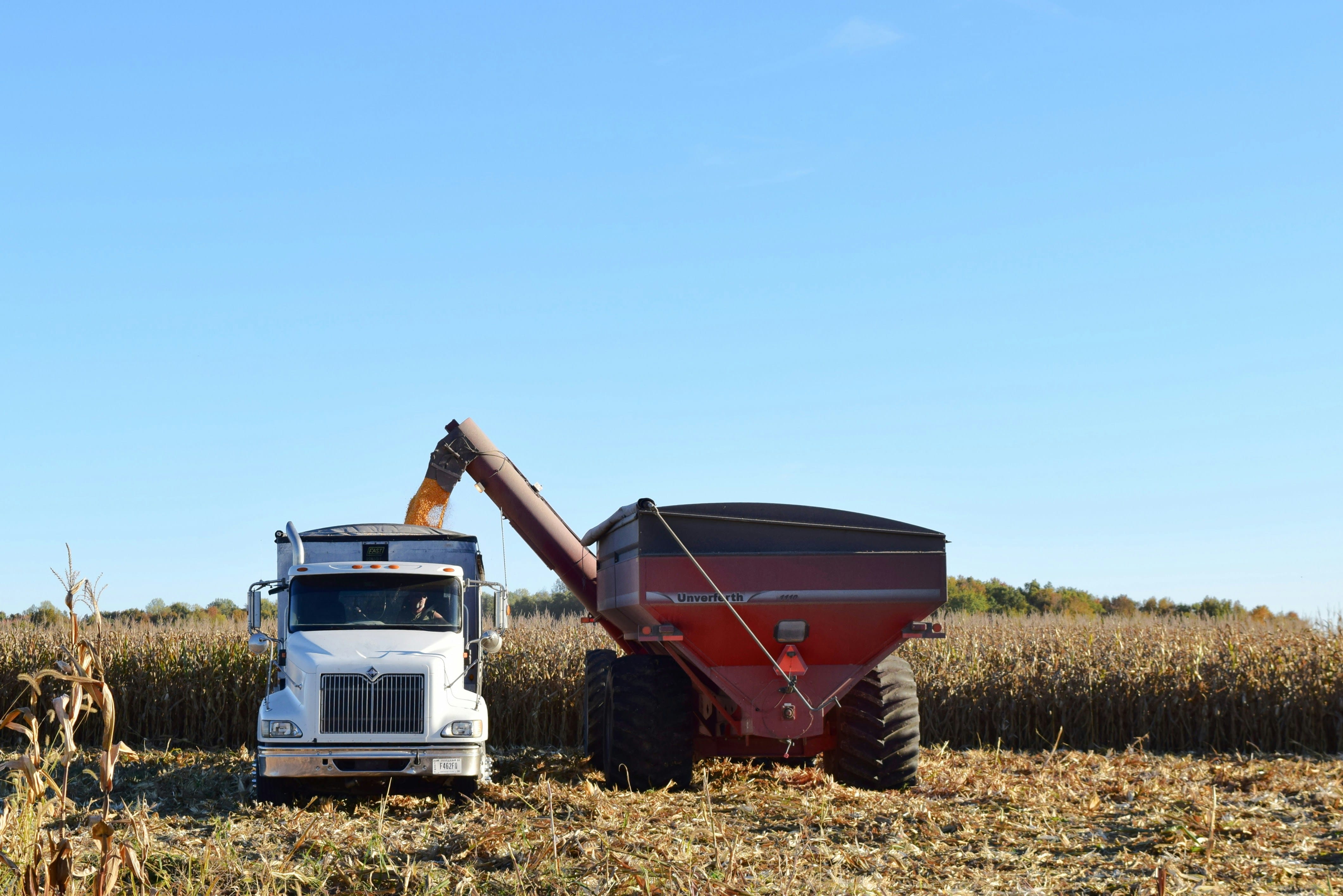
• Based on the distance of the field to the drying, storage, or purchasing facility, the crop transportation method estimates the fuel usage to transport the total crop production output. The amount of fuel is multiplied by the corresponding impact factors.

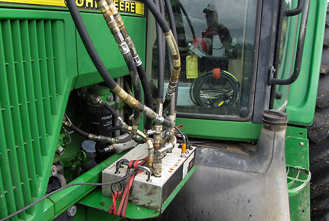
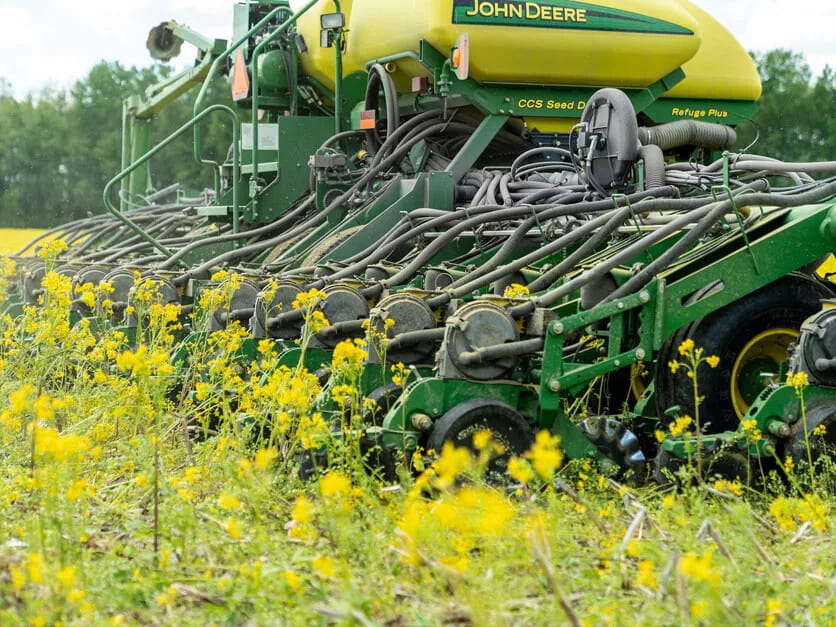
• Based on the field activities (plant, harvest, tillage, nutrient and pesticide applications, etc.), the field operations method uses the CRLMOD reference data (Kucera and Coreil 2023) to estimate the diesel fuel usage for the crop interval (crop intervals are explained here). The amount of fuel is multiplied by the corresponding impact factors.

• The crop rotation and management history, from 2008 to the latest available year, is sent to Colorado State University Cloud Services Integration Platform (David et al. 2014) to run the SWAT+ model to estimate soil carbon stock changes. Colorado State University also runs the models for the Soil Conservation and Water Quality metrics. The Soil Conservation and Water Quality metrics are not discussed at length in this document and they are not under revision.

• If a grower indicates that lime was applied, the CO₂ from carbonate lime applications to soils method is run.

• If a grower indicates that urea was applied, the CO₂ from urea fertilizer applications is run.

• If a grower indicates that crop residue was set on fire, the non-CO₂ emissions from biomass burning method is run.

• For rice production, the CH₄ emissions from flooded rice cultivation method is run.

• If direct land use change is detected, the direct land use change method is run.

• The following methods are run in all cases: CH₄ flux from non-flooded soils, soil N₂O, and soil carbon stock changes.

• For GHG emissions, disaggregated quantities of gases (CO₂, CH₄, N₂O) are multiplied by the default GWP or by the GWP selected by the grower or project.

• Once all energy use and GHG emissions are estimated at the whole-field level, the estimates are divided by area and by crop production output unit (kg, lb, bushel, etc.).

References

Arena, Marika, Giovanni Azzone, and Antonio Conte. 2013. “A Streamlined LCA Framework to Support Early Decision Making in Vehicle Development.” Journal of Cleaner Production 41: 105113.

Audsley, Eric, K. F. Stacey, David J. Parsons, and Adrian G. Williams. 2009. “Estimation of the Greenhouse Gas Emissions from Agricultural Pesticide Manufacture and Use.” https://dspace.lib.cranfield.ac.uk/handle/1826/3913.

Bandekar, Prathamesh A., Ben Putman, Greg Thoma, and Marty Matlock. 2022. “Cradle-to-Grave Life Cycle Assessment of Production and Consumption of Pulses in the United States.” Journal of Environmental Management 302 (January): 114062. https://doi.org/10.1016/j.jenvman.2021.114062.

Barber, Andrew. 2004. “Seven Case Study Farms: Total Energy & Carbon Indicators for New Zealand Arable & Outdoor Vegetable Production.” AgriLINK New Zealand Ltd 288.

BLS. 2017. “Commodity Flow Survey (CFS).” https://www.bts.gov/cfs.

Czyrnek-Delêtre, Magdalena M., Beatrice M. Smyth, and Jerry D. Murphy. 2017. “Beyond Carbon and Energy: The Challenge in Setting Guidelines for Life Cycle Assessment of Biofuel Systems.” Renewable Energy 105: 436–48. https://doi.org/https://doi.org/10.1016/j.renene.2016.11.043.

David, Olaf, Wes Lloyd, Ken Rojas, Mazdak Arabi, Frank Geter, James C Ascough II, Tim Green, George Leavesley, and Jack Carlson. 2014. “Model-as-a-Service (MaaS) Using the Cloud Services Innovation Platform (CSIP).”

European Chemicals Agency. 2024. “Search for Chemicals.” https://echa.europa.eu/information-on-chemicals.

Fava, Jim, Steven Baer, and Joyce Cooper. 2011. “Green (Er) Product Standard Trends in North America.” Journal of Industrial Ecology 15 (1): 912.

Fertilizers Europe. 2024. “Carbon Footprinting in Fertilizer Production.” https://www.fertilizerseurope.com/initiatives/carbon-footprint-calculator/.

Gaidajis, Georgios, and Ilias Kakanis. 2020. “Life Cycle Assessment of Nitrate and Compound Fertilizers Productiona Case Study.” Sustainability 13 (1): 148.

Green, MR. 1987. “Energy in Pesticide Manufacture, Distribution and Use.” Energy in Plant Nutrition and Pest Control.

Hanson, Wes L, Cortney Itle, Kara Edquist, and others. 2024. “Quantifying Greenhouse Gas Fluxes in Agriculture and Forestry: Methods for Entity-Scale Inventory.”

Heidari, Mohammad Davoud, Damien Mathis, Pierre Blanchet, and Ben Amor. 2019. “Streamlined Life Cycle Assessment of an Innovative Bio-Based Material in Construction: A Case Study of a Phase Change Material Panel.” Forests 10 (2): 160.

Hunt, Robert G, Terrie K Boguski, Keith Weitz, and Aarti Sharma. 1998. “Case Studies Examining LCA Streamlining Techniques.” The International Journal of Life Cycle Assessment 3: 3642.

IPCC. 2019. “2019 Refinement to the 2006 IPCC Guidelines for National Greenhouse Gas Inventories.”

———. 2023. “Climate Change 2023: Synthesis Report. Contribution of Working Groups i, II and III to the Sixth Assessment Report of the Intergovernmental Panel on Climate Change.” Core Writing Team, Lee, H. And Romero, J. (Eds.). https://doi.org/10.59327/IPCC/AR6-9789291691647.

ISO. 2006. “Environmental Management Life Cycle Assessment Principles and Framework.”

Kløverpris, Jesper Hedal, Claus Nordstrøm Scheel, Jannick Schmidt, Brian Grant, Ward Smith, and Murray J Bentham. 2020. “Assessing Life Cycle Impacts from Changes in Agricultural Practices of Crop Production: Methodological Description and Case Study of Microbial Phosphate Inoculant.” The International Journal of Life Cycle Assessment 25: 19912007.

Kucera, Michael J., and Christopher B. Coreil. 2023. “Overview of USDA-NRCS Erosion Prediction Technology and Conservation Resources - Land Management Operations Database and Use.” Soil Erosion Research Under a Changing Climate, January 8-13, 2023, Aguadilla, Puerto Rico, USA. https://doi.org/10.13031/soil.23007.

LEIF. 2025. “Impact Factors.” https://www.leifllc.com/.

Liu, Xinyu, Hao Cai, Hoyoung Kwon, and Michael Wang. 2023. “Feedstock Carbon Intensity Calculator (FD-CIC): Users’ Manual and Technical Documentation.”

Mendoza Beltran, Angelica, Claus Nordstrøm Scheel, Nuala Fitton, Jannick Schmidt, and Jesper Hedal Kløverpris. 2021. “Assessing Life Cycle Environmental Impacts of Inoculating Soybeans in Argentina with Bradyrhizobium Japonicum.” The International Journal of Life Cycle Assessment 26: 15701585.

National Renewable Energy Laboratory. 2012. “U.s. Life Cycle Inventory Database.” https://www.nrel.gov/analysis/lci.

Pelton, Rylie. 2018. “Spatial Greenhouse Gas Emissions from US County Corn Production.” The International Journal of Life Cycle Assessment 24 (1): 1225. https://doi.org/10.1007/s11367-018-1506-0.

Pier, F, S Trude, A Kyle, C William, D Jean-Louis, F David, DJ Lunt, et al. 2021. “Chapter 7: The Earth’s Energy Budget, Climate Feedbacks and Climate Sensitivity.” Climate Change, 132.

Pimentel, David. 2019. Handbook of Energy Utilization in Agriculture. CRC press.

Richards, Meryl B. 2018. “Measure the Chain: Tools for Assessing GHG Emissions in Agricultural Supply Chains.” https://www.ceres.org/resources/reports/measure-chain-tools-managing-ghg-emissions-agricultural-supply-chains.

Sieverding, Heidi, Ermias Kebreab, Jane M. F. Johnson, Hui Xu, Michael Wang, Stephen J. Del Grosso, Stephanie Bruggeman, et al. 2020. “A Life Cycle Analysis (LCA) Primer for the Agricultural Community.” Agronomy Journal 112 (5): 37883807. https://doi.org/10.1002/agj2.20279.

Tools, Hydrogen. 2024. “Hydrogen Analysis Resource Center (HYARC) Calculators.” https://h2tools.org/hyarc/calculator-tools/lower-and-higher-heating-values-fuels.

USDA. 2019. “Fertilizer Use and Price.” US Department of Agriculture, Economic Research Service.

USDA NASS. 2024. “Surveys: Agricultural Chemical Use Program.”

USEPA. 2023a. “GHG Emission Factors Hub.” U.S. Environmental Protection Agency. https://www.epa.gov/climateleadership/ghg-emission-factors-hub.

———. 2023b. “Inventory of u.s. Greenhouse Gas Emissions and Sinks: 1990-2021” EPA 430-R-23-002. https://www.epa.gov/ghgemissions/inventory-us-greenhouse-gas-emissions-and-sinks-1990-2021.

———. 2024. “Pesticide Product and Label System Database.” https://ordspub.epa.gov/ords/pesticides/f?p=PPLS:1.

———. 2025. “What Is Grid Gross Loss?” https://www.epa.gov/egrid/frequent-questions-about-egrid#What%20is%20Grid%20Gross%20Loss.

USEPA, OAR. 2023. “Emissions & Generation Resource Integrated Database (eGRID).” https://www.epa.gov/egrid.

Verghese, Karli L, Ralph Horne, and Andrew Carre. 2010. “PIQET: The Design and Development of an Online ‘Streamlined’LCA Tool for Sustainable Packaging Design Decision Support.” The International Journal of Life Cycle Assessment 15: 608620.

Wang, Michael, Amgad Elgowainy, Uisung Lee, Kwang Hoon Baek, Sweta Balchandani, Pahola Thathiana Benavides, Andrew Burnham, et al. 2023. “Summary of Expansions and Updates in r&d GREET 2023.” Argonne National Laboratory (ANL), Argonne, IL (United States).

Wang, Yixuan, James W Levis, and Morton A Barlaz. 2021. “Development of Streamlined Life-Cycle Assessment for the Solid Waste Management System.” Environmental Science & Technology 55 (8): 5475–84.

Footnotes

1. While the AR6 100-yr factors will be the default, Fieldprint Platform users may have the ability to choose other GWP factors.

2. Field to Market contracted with Rylie Pelton, Ph.D., to assist with the Fieldprint Platform revision. Dr. Pelton is the founder and CEO of LEIF, and a Research Scientist of Industrial Ecology at the University of Minnesota Institute on the Environment, specializing in methods to assess and improve the impacts of complex supply chains. Dr. Pelton holds a Ph.D. in Industrial Ecology, a Ph.D. minor in Public Health, and a M.S. and B.S. in Corporate Environmental Management from the University of Minnesota.

3. Users may observe that some input fields in the user interface already contain a default value. These default values were determined for each crop using literature reviews and other datasets and sources. Defaults should be replaced whenever primary data is available.