| Geographic Level | Crop | Data Category | Acres (2024) | Hectares (2024) |
|---|---|---|---|---|
| US Total | Barley | Barley - Acres Planted | 2,373,000 | 960,340 |
| US Total | Beans | Beans, Dry Edible, (Excl Chickpeas) - Acres Planted | 1,533,000 | 620,397 |
| US Total | Chickpeas | Chickpeas - Acres Planted | 502,000 | 203,157 |
| US Total | Corn | Corn - Acres Planted | 90,594,000 | 36,662,890 |
| US Total | Cotton | Cotton - Acres Planted | 11,174,000 | 4,522,056 |
| US Total | Peanuts | Peanuts - Acres Planted | 1,801,000 | 728,855 |
| US Total | Peas | Peas, Dry Edible - Acres Planted | 976,000 | 394,982 |
| US Total | Potatoes | Potatoes - Acres Planted | 930,000 | 376,366 |
| US Total | Rice | Rice - Acres Planted | 2,910,000 | 1,177,661 |
| US Total | Sorghum | Sorghum - Acres Planted | 6,300,000 | 2,549,575 |
| US Total | Soybeans | Soybeans - Acres Planted | 87,050,000 | 35,228,652 |
| US Total | Sugarbeets | Sugarbeets - Acres Planted | 1,104,300 | 446,904 |
| US Total | Wheat | Wheat - Acres Planted | 46,079,000 | 18,647,916 |
| US Total | Hay | Hay, Alfalfa - Acres Harvested | 14,612,000 | 5,913,395 |
| US Total | All Crops Above | All Above | 267,938,300 | 108,433,144 |
1 Purpose
This section includes additional details for various topics, methods, and reference data. This document contains technical information. The language used here will, at times, be repetitive to reduce ambiguity.
2 Describing the concept of crop intervals
A crop interval is defined as the period between two dates in which on-farm and field activities are conducted to produce a cash crop. Defining a crop interval is critical to creating a well-defined and continuous sequence of crop management activities for a given field.
A crop interval starts after the last day of harvest of the previous cash crop and ends with the harvest of the next cash crop. Crop drying is included in the crop interval regardless of when the drying operation is conducted. A crop interval might start on the same day of harvest when there is a field operation on that day (stalk shredding, tillage, etc.); otherwise, the crop interval starts on the day after harvest. The energy use and GHG emissions associated with on-farm and field activities that occur during the crop interval are attributed to the cash crop being produced. Crop intervals typically straddle calendar years; however, there are some exceptions, such as short-season double-crops. Crop intervals are named using the crop name and harvest year or month-year of harvest. For example, a crop interval for cotton harvested in 2023 would be named 2023 cotton or 2023-10 cotton to specify that is was harvested in October of 2023. The month-harvest designation will only be used when there are two crop harvests of the same crop in one calendar year.
To close a crop interval, the crop must result in economic gain. Economic gain is defined as crop harvest, either with machinery (grain, forage removal) or consumed by livestock on-site. Fallow years, crop failures, and crop abandonment require specific treatment; these scenarios are discussed in the sections below.
Growing a cover crop for soil cover, green manure, or other soil health benefits does not count as economic gain to define a crop interval. The energy use and GHG emissions associated with cover cropping activities are attributed to the following cash crop.
Below, we include eight scenarios to illustrate the concept of crop intervals. To be concise, we show a simplified list of field activities, omitting crop transportation, drying, and irrigation events, along with other operations.
2.1 Case 1: A grower produces one cash crop per season
In the simplest case, a crop interval starts after the harvest of the previous cash crop and ends with the harvest of the following cash crop.
The following figure demonstrates the crop intervals for a corn-soybean rotation.
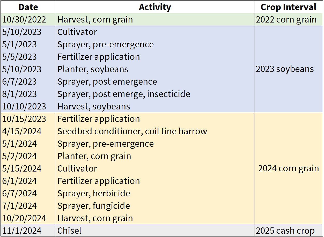
In Case 1, the energy use and GHG emissions associated with the field activities after the harvest of the 2022 corn grain are attributed to the 2023 soybean crop, the energy use and GHG emissions associated with the activities after harvest of soybeans are attributed to the 2024 corn crop, and so on. For the two crops with complete information shown above, the crop intervals would be delineated as follows:
- 2023 soybeans, 10-31-2022 to 10-10-2023
- 2024 corn grain, 10-11-2023 to 10-20-2024
2.2 Case 2: A grower has a rotation with double-cropping
In many regions of the US, growers can add a second, short-season crop to their rotations. A common double-crop rotation is producing soybeans after a winter wheat harvest.
The following figure demonstrates the crop intervals for a rotation with double-cropping.
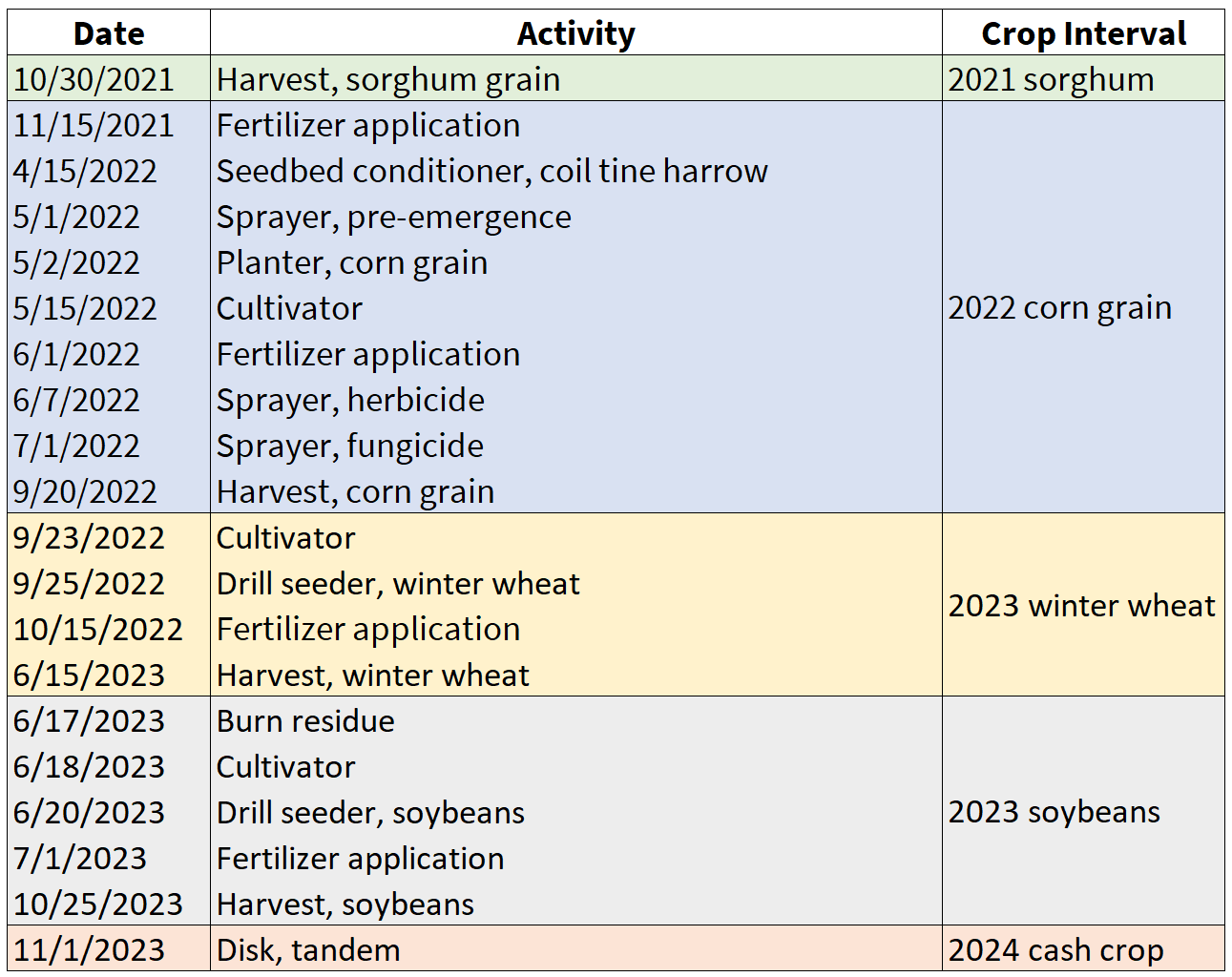
In this rotation, the 2023 soybeans have a short crop interval that lasts around four months without straddling a calendar year. For the crops with complete information shown above, the crop intervals would be delineated as follows:
- 2022 corn grain: 10/31/2021 to 9/20/2022
- 2023 winter wheat: 9/21/2022 to 6/15/2023
- 2023 soybeans: 6/16/2023 to 10/15/2023
The energy use and GHG emissions associated with the on-farm and field activities within the dates of the crop interval are attributed to the cash crop named in the crop interval.
2.3 Case 3: A grower produces a cash crop per year and adds cover cropping
In this case, a grower introduces cover crops to the rotation while harvesting one cash crop per year. The cover cropping activities (planting, seed inputs, chemical or mechanical termination, etc.) are included in the crop interval for the cash crop.
The following figure demonstrates the crop intervals for a rotation with cash crops and cover crops.
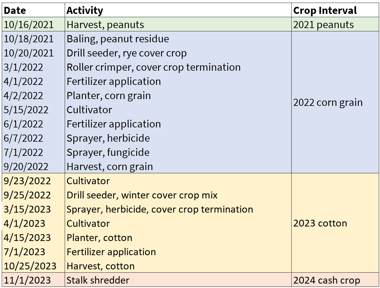
As before, the energy use and GHG emissions associated with the on-farm and field activities are attributed to the crop named in the crop interval. If the cover crop were to be harvested for forage or grain, or if it was consumed by livestock, that would make it a cash crop, and the crop interval would be named and delineated accordingly.
For the crops with complete information shown above, the crop intervals would be delineated as follows:
- 2022 corn grain: 10/17/2021 to 9/20/2022
- 2023 cotton: 9/21/2022 to 10/25/2023
2.4 Case 4: A grower has fallow years in the rotation
Fallow cropping is common in dryland systems in many regions of the US, including the Great Plains, the Pacific Northwest, and the Rocky Mountain region. Fallow cropping refers to leaving a field unplanted during one or more growing seasons. This is typically done to build up soil water reserves for the following cash crop, among other reasons. Fallow years might have light tillage operations or applications of herbicides to control weeds. The energy use and GHG emissions of those activities, plus any estimated soil N2O emissions or other sources of emissions, are attributed to the following cash crop.
The following figure demonstrates the crop intervals for a rotation with fallow cropping.
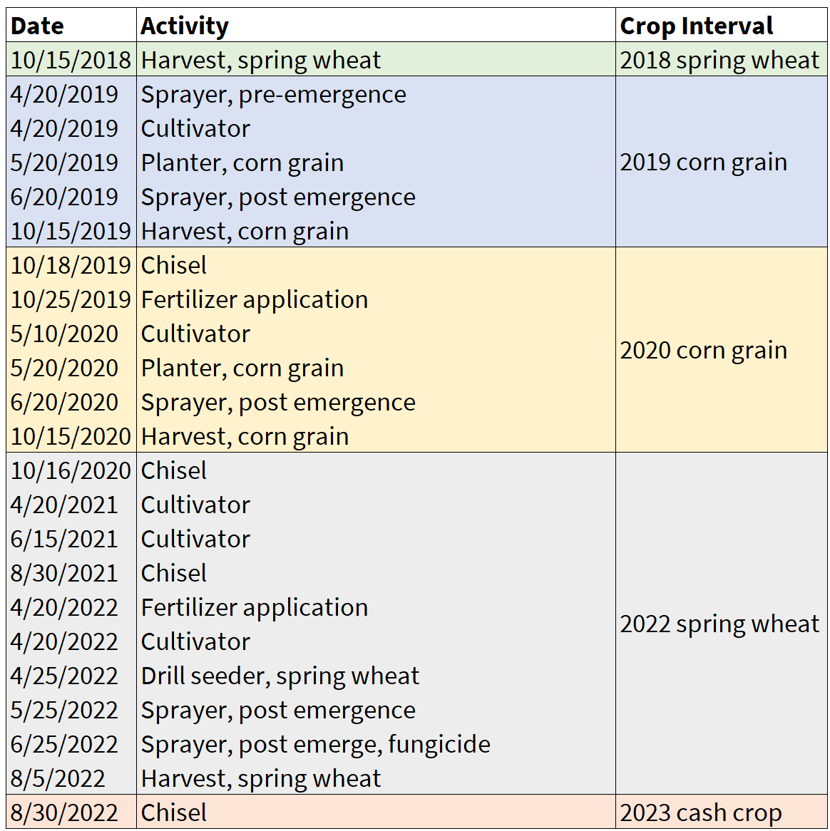
In the example above, 2021 is a fallow year with multiple light tillage passes to control weeds. The 2022 spring wheat crop interval spans two years. For the crops with complete information shown above, the crop intervals would be delineated as follows:
- 2019 corn grain: 10/16/2018 to 10/15/2019
- 2020 corn grain: 10/16/2019 to 10/15/2020
- 2022 spring wheat: 10/16/2020 to 8/5/2022
2.5 Case 5: A grower experiences crop failure or crop abandonment
In the unfortunate case in which a crop is killed by weather events, such as hail, flood, or drought, the on-farm and field activities for the failed or abandoned crop are assigned to the following cash crop. This is similar to how fallow cropping is treated.
The following figure demonstrates the crop intervals for a rotation with a failed crop.
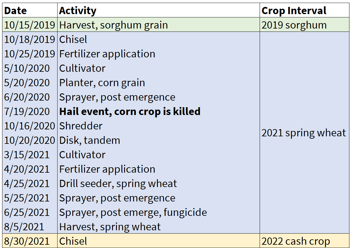
In the example above, the 2020 corn crop suffered a hail event that killed the growing crop (the event is shown in bold font). The grower shredded and incorporated the corn biomass into the soil and returned in the 2021 season to grow spring wheat. The energy use and GHG emissions associated with the failed corn crop are attributed to the 2021 spring wheat.
For the crops with complete information shown above, the crop intervals would be delineated as follows:
- 2021 spring wheat: 10/16/2019 to 8/5/2021
2.6 Case 6: A grower produces a rice crop with ratooning
Rice producers, mostly in Texas and Louisiana, can benefit from harvesting two rice crops from the same planted seeds. This presents a unique situation for which there is little guidance for GHG emission accounting methodologies, and it blurs the lines of crop interval delineation. We are faced with three complications:
- The method for CH4 emissions from flooded rice cultivation, as published by Ogle et al. (2024), does not contain guidance about how to account for ratoon emissions.
- Rice ratooning cannot be classified strictly as a double crop because it is harvested from the regrowth of the first rice crop planted at the beginning of the season. It is also not a given that both crops will be managed with the same level of inputs, such as fertilizers.
- The guidance published in IPCC (2019) indicates that the area harvested for the main crop and the ratoon crop should be summed together, which leads to having to sum together the crop production outputs from the two harvests (primary rice crop + ratoon crop).
To solve these challenges, Field to Market proposes using the following approach until better guidance emerges:
- If a field produces annual rice with no ratooning, the method CH4 emissions from flooded rice cultivation is run, and the accounting of energy use and GHG emissions is similar to an annual cash crop described in Section 2.1.
- If a field produces rice with a ratoon crop, the method CH4 emissions from flooded rice cultivation is run aggregating inputs and outputs for both rice crops, and extending the season length from the planting of the first rice crop to the harvest of the ratoon crop (approximately 133 days + 60 days). The estimated energy use and GHG emissions are representative of both crops. This will require filling in some assumptions. Taking this approach will typically result in higher emissions per area (e.g., kg CO2e / ha) and lower emissions per crop production unit (e.g., kg CO2e / kg rice crop) compared to producing a single rice crop per year.
The following figure demonstrates the crop intervals for a rotation with rice ratooning. To be concise, many field activities were omitted from the timeline of operations.
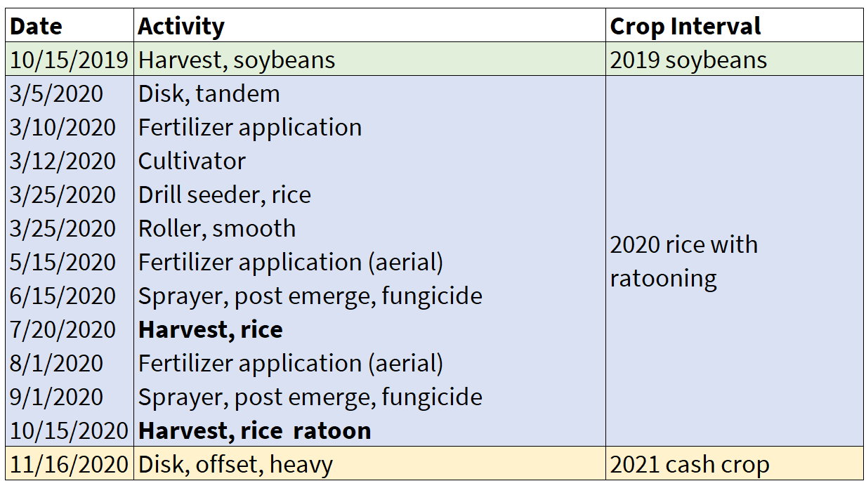
For the crops with complete information shown above, the crop intervals would be delineated as follows:
- 2020 rice with ratooning: 10/16/2019 to 10/15/2020
2.7 Case 7: A grower has a rotation with multi-year alfalfa and annual crops
Alfalfa is currently the only perennial crop in Field to Market’s programs. In addition, alfalfa can be harvested multiple times per growing season. The Fieldprint Platform needs the following rules to account for crop intervals for alfalfa:
- The first crop interval for alfalfa will start after the harvest of the last cash crop, and end after the last harvest of the first year with biomass removal. The first crop interval will typically span two years, since the first establishment year is unlikely to include any biomass harvesting.
- For the rest of the alfalfa stand, crop intervals will start after the last harvest in the previous calendar year, and end with the last harvest in the following year. After the first establishment crop interval, all other intervals will accumulate the multiple harvests conducted in a given calendar year.
The following figure demonstrates the crop intervals for a rotation with alfalfa. To be concise, many field activities were omitted from the timeline of operations. Alfalfa was planted in August 2015, and the first harvest occurred in the spring of 2016.
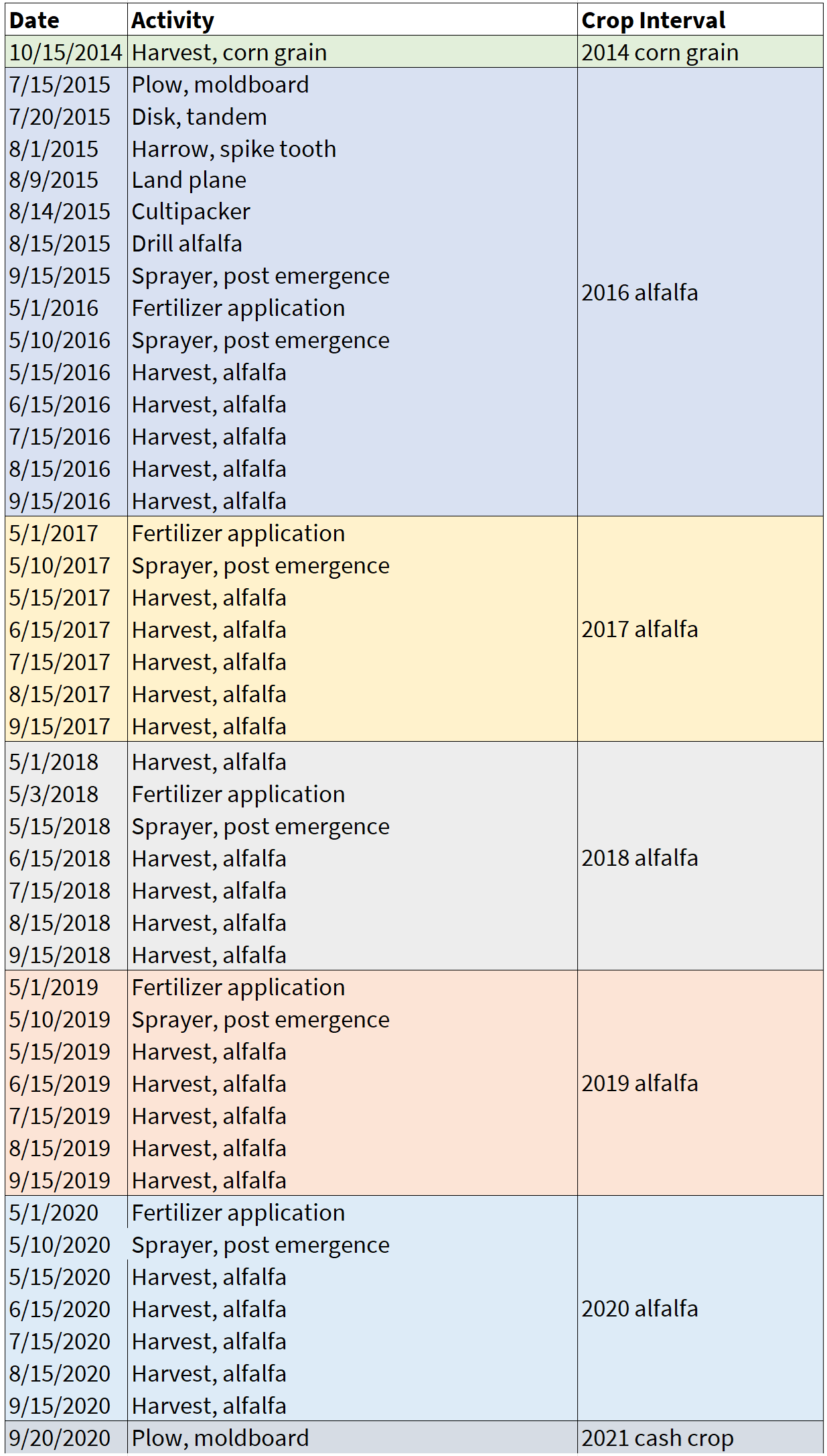
To illustrate the first two crop intervals, the delineation would be as follows:
- 2026 alfalfa: 10/16/2014 to 9/15/2016. This includes the establishment year (2015) and five biomass harvests in 2016.
- 2017 alfalfa: 9/16/2016 to 9/15/2017. This includes five biomass harvests.
Alfalfa crop intervals will continue in the same manner until the crop is terminated, either mechanically with heavy plowing or a mix of tillage and chemical applications. In the example above, the alfalfa stand produced 25 biomass harvests in the span of six years.
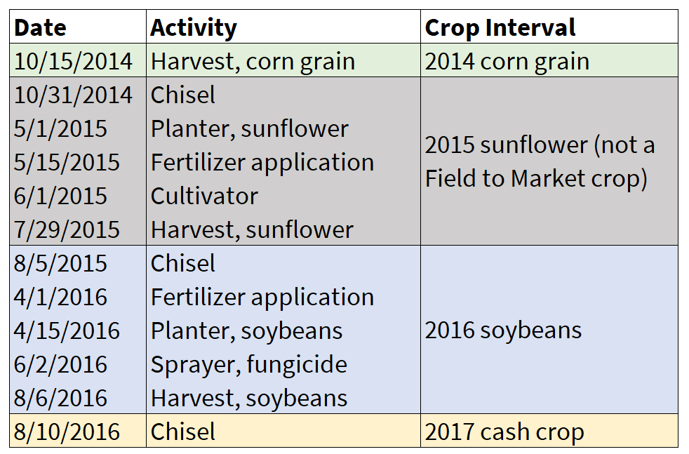
2.8 Case 8: Fields with rotations that include crops not part of Field to Market’s program
For FP v5, the system will fill the crop rotation sequence for a given field from 2008 to the latest available year using the Cropland Data Layer (Boryan et al. 2011). This will bring crops that are not yet part of Field to Market’s programs. We will use the crop rotation to model soil carbon stock changes and soil erosion; however, the FP v5 cannot produce output for energy use and GHG emissions for those crop intervals.
The following figure demonstrates a crop interval with a non-FTM crop.
3 Area planted or harvested for Field to Market crops
In 2024, USDA NASS surveys reported the following area planted (area harvested for alfalfa) for the crops in Field to Market’s program. The Fieldprint Platform can be used to quantify the impact of approximately 267 million acres (108 million hectares) of United States cropland.
4 Global Warming Potential factors
In FP v5, individual growers and project administrators aggregating grower data will be able to select the Global Warming Potential (GWP) factor that meets their needs.
Biogenic CO2, excluding emissions from direct land use change and soil carbon stock changes, can be manually removed by users, since those emissions are part of the natural carbon cycle.
The default GWP will be AR6 with 100-yr horizon:
| Assessment Report (AR) | Time Horizon | Gas | Global Warming Potential |
|---|---|---|---|
| AR6 | 100-yr | CO2_fossil | 1.0 |
| AR6 | 100-yr | CO2_biogenic | 1.0 |
| AR6 | 100-yr | CH4_biogenic | 27.0 |
| AR6 | 100-yr | CH4_fossil | 29.8 |
| AR6 | 100-yr | N2O | 273.0 |
| AR6 | 100-yr | NF3 | 17400.0 |
| AR6 | 100-yr | SF6 | 25200.0 |
Including the default factors shown above, the following options will be available for 100- and 20-yr horizons:
| Assessment Report (AR) |
|---|
| AR6 |
| AR5 (with climate-carbon feedback) |
| AR5 (without climate-carbon feedback) |
| AR4 |
The complete list of GWP factors is shown in the table below.
| Assessment Report (AR) | Time Horizon | Gas | Global Warming Potential |
|---|---|---|---|
| AR6 | 100-yr | CO2_fossil | 1.0 |
| AR6 | 100-yr | CO2_biogenic | 1.0 |
| AR6 | 100-yr | CH4_biogenic | 27.0 |
| AR6 | 100-yr | CH4_fossil | 29.8 |
| AR6 | 100-yr | N2O | 273.0 |
| AR6 | 100-yr | NF3 | 17400.0 |
| AR6 | 100-yr | SF6 | 25200.0 |
| AR5 (with climate-carbon feedback) | 100-yr | CO2_fossil | 1.0 |
| AR5 (with climate-carbon feedback) | 100-yr | CO2_biogenic | 1.0 |
| AR5 (with climate-carbon feedback) | 100-yr | CH4_biogenic | 34.0 |
| AR5 (with climate-carbon feedback) | 100-yr | CH4_fossil | 36.0 |
| AR5 (with climate-carbon feedback) | 100-yr | N2O | 298.0 |
| AR5 (with climate-carbon feedback) | 100-yr | NF3 | 17885.0 |
| AR5 (with climate-carbon feedback) | 100-yr | SF6 | 26087.0 |
| AR5 (without climate-carbon feedback) | 100-yr | CO2_fossil | 1.0 |
| AR5 (without climate-carbon feedback) | 100-yr | CO2_biogenic | 1.0 |
| AR5 (without climate-carbon feedback) | 100-yr | CH4_biogenic | 28.0 |
| AR5 (without climate-carbon feedback) | 100-yr | CH4_fossil | 30.0 |
| AR5 (without climate-carbon feedback) | 100-yr | N2O | 265.0 |
| AR5 (without climate-carbon feedback) | 100-yr | NF3 | 16100.0 |
| AR5 (without climate-carbon feedback) | 100-yr | SF6 | 23500.0 |
| AR4 | 100-yr | CO2_fossil | 1.0 |
| AR4 | 100-yr | CO2_biogenic | 1.0 |
| AR4 | 100-yr | CH4_biogenic | 25.0 |
| AR4 | 100-yr | CH4_fossil | 25.0 |
| AR4 | 100-yr | N2O | 298.0 |
| AR4 | 100-yr | NF3 | 17200.0 |
| AR4 | 100-yr | SF6 | 22800.0 |
| AR6 | 20-yr | CO2_fossil | 1.0 |
| AR6 | 20-yr | CO2_biogenic | 1.0 |
| AR6 | 20-yr | CH4_biogenic | 79.7 |
| AR6 | 20-yr | CH4_fossil | 82.5 |
| AR6 | 20-yr | N2O | 273.0 |
| AR6 | 20-yr | NF3 | 13400.0 |
| AR6 | 20-yr | SF6 | 18300.0 |
| AR5 (with climate-carbon feedback) | 20-yr | CO2_fossil | 1.0 |
| AR5 (with climate-carbon feedback) | 20-yr | CO2_biogenic | 1.0 |
| AR5 (with climate-carbon feedback) | 20-yr | CH4_biogenic | 86.0 |
| AR5 (with climate-carbon feedback) | 20-yr | CH4_fossil | 87.0 |
| AR5 (with climate-carbon feedback) | 20-yr | N2O | 268.0 |
| AR5 (with climate-carbon feedback) | 20-yr | NF3 | 13008.0 |
| AR5 (with climate-carbon feedback) | 20-yr | SF6 | 17783.0 |
| AR5 (without climate-carbon feedback) | 20-yr | CO2_fossil | 1.0 |
| AR5 (without climate-carbon feedback) | 20-yr | CO2_biogenic | 1.0 |
| AR5 (without climate-carbon feedback) | 20-yr | CH4_biogenic | 84.0 |
| AR5 (without climate-carbon feedback) | 20-yr | CH4_fossil | 85.0 |
| AR5 (without climate-carbon feedback) | 20-yr | N2O | 264.0 |
| AR5 (without climate-carbon feedback) | 20-yr | NF3 | 12800.0 |
| AR5 (without climate-carbon feedback) | 20-yr | SF6 | 17500.0 |
| AR4 | 20-yr | CO2_fossil | 1.0 |
| AR4 | 20-yr | CO2_biogenic | 1.0 |
| AR4 | 20-yr | CH4_biogenic | 72.0 |
| AR4 | 20-yr | CH4_fossil | 72.0 |
| AR4 | 20-yr | N2O | 289.0 |
| AR4 | 20-yr | NF3 | 12300.0 |
| AR4 | 20-yr | SF6 | 16300.0 |
5 Impact factors
Impact factors represent the cumulative energy demand (CED) and associated GHG emissions with manufacturing a unit of output for a given category, such as a kg of fertilizer, a MWh of electricity, a gallon of fuel, etc.
The impact factors are as follows.
5.1 Electricity
Due to a data restriction, Field to Market is unable to post the electricity impact factors here; however, we are able to present the data to interested reviewers.
In broad terms, electricity factors represent 27 energy grids in the United States, and include the cumulative energy demand and associated GHG emissions for electricity generation, transmission, and distribution. The electric grid selected is tied to the field location entered by a user.
In the FP v5, electricity impact factors are used by two farming operations:
- Irrigation operations
- Crop drying
5.2 Fuels
For FP v5, the fuel options have been reduced and tied to specific operations. We have also incorporated more reliable data and separated the impact factors by on-farm combustion and upstream manufacturing impacts for the procured fuel.
The FP v5 won’t include biogenic CO2 from biofuels in the final estimate for the GHG Emissions metric, as permitted by the Greenhouse Gas Reporting Program (GHGRP).
The fuels are linked to operations as follows:
- Irrigation pumping
- Diesel (ag equipment)
- Gasoline
- LPG
- Natural gas
- Crop drying
- Diesel (ag equipment)
- Gasoline
- LPG
- Natural gas
- Crop transportation
- Biodiesel (on-road heavy-duty truck). This is based on B100.
- Diesel (on-road medium-heavy duty truck)
- Manure transportation
- Diesel (on-road medium-heavy duty truck)
- Field operations
- Diesel (ag equipment)
- Agricultural input transportation
- Diesel (on-road medium-heavy duty truck)
5.2.1 Energy use
The energy use impact factors are explained below.
- System Boundary: This enables the disaggregation of upstream and combustion factors. Combustion factors are attributed to On-Farm Mechanical or Post-harvest boundaries. The combustion factors for On-Farm Mechanical or Post-harvest are the same.
- Source Category: It classifies the energy use to indicate whether it is associated with production of fuels (upstream), mobile machinery (field equipment, crop transportation, manure transportation), and stationary machinery (irrigation pumps and crop dryers).
- Source: A given fuel.
- MJ: Impact factor of megajoules per unit.
- Unit (LHV): Expected unit to use the MJ impact factor.
The energy use impact factors are given below.
| System Boundary | Source Category | Source | MJ | Unit (LHV) |
|---|---|---|---|---|
| Upstream | Energy use associated with production of fuels | Biodiesel (on-road heavy-duty truck) | 74.34 | gallon |
| Upstream | Energy use associated with production of fuels | Diesel (ag equipment) | 15.94 | gallon |
| Upstream | Energy use associated with production of fuels | Diesel (on-road medium-heavy duty truck) | 15.94 | gallon |
| Upstream | Energy use associated with production of fuels | Gasoline | 26.93 | gallon |
| Upstream | Energy use associated with production of fuels | LPG | 12.70 | gallon |
| Upstream | Energy use associated with production of fuels | Natural gas | 0.11 | SCF |
| Upstream | Energy use associated with transportation of agricultural inputs | Diesel (on-road medium-heavy duty truck) | 160.88 | gallon |
| Post-Harvest | Energy use associated with mobile machinery | Diesel (on-road medium-heavy duty truck) | 144.94 | gallon |
| Post-Harvest | Energy use associated with mobile machinery | Biodiesel (on-road heavy-duty truck) | 126.13 | gallon |
| Post-Harvest | Energy use associated with stationary machinery | Diesel (ag equipment) | 144.94 | gallon |
| Post-Harvest | Energy use associated with stationary machinery | Gasoline | 118.29 | gallon |
| Post-Harvest | Energy use associated with stationary machinery | LPG | 88.89 | gallon |
| Post-Harvest | Energy use associated with stationary machinery | Natural gas | 1.08 | SCF |
| On-Farm Mechanical | Energy use associated with mobile machinery | Diesel (ag equipment) | 144.94 | gallon |
| On-Farm Mechanical | Energy use associated with mobile machinery | Diesel (on-road medium-heavy duty truck) | 144.94 | gallon |
| On-Farm Mechanical | Energy use associated with mobile machinery | Biodiesel (on-road heavy-duty truck) | 126.13 | gallon |
| On-Farm Mechanical | Energy use associated with stationary machinery | Diesel (ag equipment) | 144.94 | gallon |
| On-Farm Mechanical | Energy use associated with stationary machinery | Gasoline | 118.29 | gallon |
| On-Farm Mechanical | Energy use associated with stationary machinery | LPG | 88.89 | gallon |
| On-Farm Mechanical | Energy use associated with stationary machinery | Natural gas | 1.08 | SCF |
5.2.2 GHG emissions
The GHG emissions impact factors are explained below.
- System Boundary: This enables the disaggregation of upstream and combustion factors. Combustion factors are attributed to On-Farm Mechanical or Post-harvest boundaries. The combustion factors for On-Farm Mechanical or Post-harvest are the same.
- Source Category: It classifies the GHG emissions to indicate whether it is associated with production of fuels (upstream), mobile machinery (field equipment, crop transportation, manure transportation), and stationary machinery (irrigation pumps and crop dryers).
- Source: A given fuel.
- CO2_fossil: Impact factor for fossil CO2 in kg of gas per unit.
- CO2_biogenic: Impact factor for biogenic CO2 in kg of gas per unit. It is important to note that the Greenhouse Gas Reporting Program (GHGRP) allows for the non-inclusion of biogenic CO2 from inventories, except for those CO2 emissions from direct land use change and soil carbon stock changes.
- CH4_fossil: Impact factor of fossil CH4 in kg of gas per unit.
- CH4_biogenic: Impact factor of biogenic CH4 in kg of gas per unit.
- N2O: Impact factor for N2O in kg of gas per unit.
- Unit (LHV): Expected unit to use the impact factors for each GHG gas.
The GHG emission impact factors are given below.
| System Boundary | Source Category | Source | CO2_fossil | CO2_biogenic | CH4_fossil | CH4_biogenic | N2O | Unit (LHV) |
|---|---|---|---|---|---|---|---|---|
| Upstream | GHG emissions associated with production of fuels | Biodiesel (on-road heavy-duty truck) | 2.24 | 0.00 | 0.0037037 | 0.00e+00 | 0.0010976 | gallon |
| Upstream | GHG emissions associated with production of fuels | Diesel (ag equipment) | 0.97 | 0.00 | 0.0023290 | 0.00e+00 | 0.0000195 | gallon |
| Upstream | GHG emissions associated with production of fuels | Diesel (on-road medium-heavy duty truck) | 0.97 | 0.00 | 0.0023290 | 0.00e+00 | 0.0000195 | gallon |
| Upstream | GHG emissions associated with production of fuels | Gasoline | 1.68 | 0.00 | 0.0046768 | 0.00e+00 | 0.0003232 | gallon |
| Upstream | GHG emissions associated with production of fuels | LPG | 0.91 | 0.00 | 0.0025506 | 0.00e+00 | 0.0000152 | gallon |
| Upstream | GHG emissions associated with production of fuels | Natural gas | 0.01 | 0.00 | 0.0001952 | 0.00e+00 | 0.0000013 | SCF |
| Upstream | GHG emissions associated with transportation of agricultural inputs | Diesel (on-road medium-heavy duty truck) | 11.18 | 0.00 | 0.0032384 | 0.00e+00 | 0.0003245 | gallon |
| Post-Harvest | GHG emissions associated with transportation of crop production | Biodiesel (on-road heavy-duty truck) | 0.00 | 9.48 | 0.0000000 | 9.95e-05 | 0.0000142 | gallon |
| Post-Harvest | GHG emissions associated with transportation of crop production | Diesel (on-road medium-heavy duty truck) | 10.20 | 0.00 | 0.0009094 | 0.00e+00 | 0.0003050 | gallon |
| Post-Harvest | GHG emissions associated with stationary machinery | Diesel (ag equipment) | 10.20 | 0.00 | 0.0012692 | 0.00e+00 | 0.0010693 | gallon |
| Post-Harvest | GHG emissions associated with stationary machinery | Gasoline | 8.72 | 0.00 | 0.0003727 | 0.00e+00 | 0.0000745 | gallon |
| Post-Harvest | GHG emissions associated with stationary machinery | LPG | 5.64 | 0.00 | 0.0002744 | 0.00e+00 | 0.0000549 | gallon |
| Post-Harvest | GHG emissions associated with stationary machinery | Natural gas | 0.05 | 0.00 | 0.0000010 | 0.00e+00 | 0.0000001 | SCF |
| On-Farm Mechanical | GHG emissions associated with mobile machinery | Diesel (ag equipment) | 10.20 | 0.00 | 0.0012692 | 0.00e+00 | 0.0010693 | gallon |
| On-Farm Mechanical | GHG emissions associated with transportation of crop production | Biodiesel (on-road heavy-duty truck) | 0.00 | 9.48 | 0.0000000 | 9.95e-05 | 0.0000142 | gallon |
| On-Farm Mechanical | GHG emissions associated with transportation of crop production | Diesel (on-road medium-heavy duty truck) | 10.20 | 0.00 | 0.0009094 | 0.00e+00 | 0.0003050 | gallon |
| On-Farm Mechanical | GHG emissions associated with stationary machinery | Diesel (ag equipment) | 10.20 | 0.00 | 0.0012692 | 0.00e+00 | 0.0010693 | gallon |
| On-Farm Mechanical | GHG emissions associated with stationary machinery | Gasoline | 8.72 | 0.00 | 0.0003727 | 0.00e+00 | 0.0000745 | gallon |
| On-Farm Mechanical | GHG emissions associated with stationary machinery | LPG | 5.64 | 0.00 | 0.0002744 | 0.00e+00 | 0.0000549 | gallon |
| On-Farm Mechanical | GHG emissions associated with stationary machinery | Natural gas | 0.05 | 0.00 | 0.0000010 | 0.00e+00 | 0.0000001 | SCF |
| On-Farm Mechanical | GHG emissions associated with mobile machinery | Diesel (on-road medium-heavy duty truck) | 10.20 | 0.00 | 0.0009094 | 0.00e+00 | 0.0003050 | gallon |
5.3 Fertilizers
For FP v5, fertilizers have been enhanced with more reliable data and better options compared to FP v4.2. The impact factors for fertilizers in this section are associated with the energy use and GHG emissions from the manufacturing process, and these impacts are attributed to the Upstream boundary. The soil GHG emissions related to the use of nitrogen fertilizers, lime, and urea are accounted by methods from Ogle et al. (2024).
5.3.1 Energy use
The energy use impact factors are described below.
- System Boundary: The impact factors in this section are attributed to the Upstream boundary.
- Source Category: It classifies the energy use to indicate it is associated with the production of fertilizers.
- Source Detail: A given fertilizer option.
- MJ: Impact factor of megajoules per unit.
- Unit: Expected unit to use the MJ impact factor.
The energy use impact factors are given below.
| System Boundary | Source Category | Source Detail | MJ | Unit |
|---|---|---|---|---|
| Upstream | Energy use associated with production of fertilizers | Ammonia (aqueous) | 0.01 | kg fertilizer |
| Upstream | Energy use associated with production of fertilizers | Ammonia (aqueous) (green ammonia) | 0.01 | kg fertilizer |
| Upstream | Energy use associated with production of fertilizers | Ammonia (conventional) | 37.75 | kg fertilizer |
| Upstream | Energy use associated with production of fertilizers | Ammonia (green) | 43.27 | kg fertilizer |
| Upstream | Energy use associated with production of fertilizers | Ammonium nitrate | 14.70 | kg fertilizer |
| Upstream | Energy use associated with production of fertilizers | Ammonium nitrate (green ammonia) | 15.87 | kg fertilizer |
| Upstream | Energy use associated with production of fertilizers | Ammonium sulfate | 18.04 | kg fertilizer |
| Upstream | Energy use associated with production of fertilizers | Ammonium sulfate (green ammonia) | 19.47 | kg fertilizer |
| Upstream | Energy use associated with production of fertilizers | Calcium ammonium nitrate | 13.66 | kg fertilizer |
| Upstream | Energy use associated with production of fertilizers | Calcium ammonium nitrate (green ammonia) | 14.48 | kg fertilizer |
| Upstream | Energy use associated with production of fertilizers | Diammonium phosphate | 23.91 | kg fertilizer |
| Upstream | Energy use associated with production of fertilizers | Diammonium phosphate (green ammonia) | 25.14 | kg fertilizer |
| Upstream | Energy use associated with production of fertilizers | Gypsum | 0.00 | kg fertilizer |
| Upstream | Energy use associated with production of fertilizers | K2O | 8.73 | kg K2O |
| Upstream | Energy use associated with production of fertilizers | Lime (calcitic) | 0.03 | kg fertilizer |
| Upstream | Energy use associated with production of fertilizers | Lime (dolomitic) | 0.03 | kg fertilizer |
| Upstream | Energy use associated with production of fertilizers | Micronutrient (boron) | 12.15 | kg fertilizer |
| Upstream | Energy use associated with production of fertilizers | Micronutrient (manganese) | 28.84 | kg fertilizer |
| Upstream | Energy use associated with production of fertilizers | Micronutrient (zinc) | 32.32 | kg fertilizer |
| Upstream | Energy use associated with production of fertilizers | Monoammonium phosphate | 22.41 | kg fertilizer |
| Upstream | Energy use associated with production of fertilizers | Monoammonium phosphate (green ammonia) | 23.16 | kg fertilizer |
| Upstream | Energy use associated with production of fertilizers | Potash (MOP) | 5.24 | kg fertilizer |
| Upstream | Energy use associated with production of fertilizers | Potassium nitrate | 14.94 | kg fertilizer |
| Upstream | Energy use associated with production of fertilizers | Sulfur | 6.64 | kg fertilizer |
| Upstream | Energy use associated with production of fertilizers | US average nitrogen fertilizer | 55.42 | kg N |
| Upstream | Energy use associated with production of fertilizers | US average phosphate fertilizer | 48.18 | kg P2O5 |
| Upstream | Energy use associated with production of fertilizers | Urea | 28.22 | kg fertilizer |
| Upstream | Energy use associated with production of fertilizers | Urea (green ammonia) | 39.74 | kg fertilizer |
| Upstream | Energy use associated with production of fertilizers | Urea ammonium nitrate | 53.58 | kg fertilizer |
| Upstream | Energy use associated with production of fertilizers | Urea ammonium nitrate (green ammonia) | 67.82 | kg fertilizer |
5.3.2 GHG emissions
The GHG emission impact factors are described below.
- System Boundary: The impact factors in this section are attributed to the Upstream boundary.
- Source Category: It classifies the GHG emissions to indicate they are associated with the production of fertilizers.
- Source Detail: A given fertilizer option.
- CO2_fossil: Impact factor for fossil CO2 in kg of gas per unit.
- CH4_fossil: Impact factor of fossil CH4 in kg of gas per unit.
- N2O: Impact factor for N2O in kg of gas per unit.
- Unit: Expected unit to use the GHG emissions impact factor.
The GHG emission impact factors are given below.
| System Boundary | Source Category | Source Detail | CO2_fossil | CH4_fossil | N2O | Unit |
|---|---|---|---|---|---|---|
| Upstream | GHG emissions associated with production of fertilizers | Ammonia (aqueous) | 0.54 | 0.0015586 | 0.0000095 | kg fertilizer |
| Upstream | GHG emissions associated with production of fertilizers | Ammonia (aqueous) (green ammonia) | 0.03 | 0.0000610 | 0.0000006 | kg fertilizer |
| Upstream | GHG emissions associated with production of fertilizers | Ammonia (conventional) | 2.16 | 0.0062343 | 0.0000381 | kg fertilizer |
| Upstream | GHG emissions associated with production of fertilizers | Ammonia (green) | 0.05 | 0.0001044 | 0.0000010 | kg fertilizer |
| Upstream | GHG emissions associated with production of fertilizers | Ammonium nitrate | 0.24 | 0.0061190 | 0.0037640 | kg fertilizer |
| Upstream | GHG emissions associated with production of fertilizers | Ammonium nitrate (green ammonia) | 0.20 | 0.0048329 | 0.0037565 | kg fertilizer |
| Upstream | GHG emissions associated with production of fertilizers | Ammonium sulfate | 0.14 | 0.0016980 | 0.0000109 | kg fertilizer |
| Upstream | GHG emissions associated with production of fertilizers | Ammonium sulfate (green ammonia) | 0.10 | 0.0001405 | 0.0000019 | kg fertilizer |
| Upstream | GHG emissions associated with production of fertilizers | Calcium ammonium nitrate | 0.45 | 0.0022787 | 0.0000544 | kg fertilizer |
| Upstream | GHG emissions associated with production of fertilizers | Calcium ammonium nitrate (green ammonia) | 0.14 | 0.0013677 | 0.0000489 | kg fertilizer |
| Upstream | GHG emissions associated with production of fertilizers | Diammonium phosphate | 0.84 | 0.0029129 | 0.0000262 | kg fertilizer |
| Upstream | GHG emissions associated with production of fertilizers | Diammonium phosphate (green ammonia) | 0.80 | 0.0015764 | 0.0000185 | kg fertilizer |
| Upstream | GHG emissions associated with production of fertilizers | Gypsum | 0.03 | 0.0000462 | 0.0000002 | kg fertilizer |
| Upstream | GHG emissions associated with production of fertilizers | K2O | 0.45 | 0.0009157 | 0.0000068 | kg K2O |
| Upstream | GHG emissions associated with production of fertilizers | Lime (calcitic) | 0.01 | 0.0000114 | 0.0000000 | kg fertilizer |
| Upstream | GHG emissions associated with production of fertilizers | Lime (dolomitic) | 0.01 | 0.0000114 | 0.0000000 | kg fertilizer |
| Upstream | GHG emissions associated with production of fertilizers | Micronutrient (boron) | 0.47 | 0.0009837 | 0.0001148 | kg fertilizer |
| Upstream | GHG emissions associated with production of fertilizers | Micronutrient (manganese) | 1.78 | 0.0029312 | 0.0002378 | kg fertilizer |
| Upstream | GHG emissions associated with production of fertilizers | Micronutrient (zinc) | 1.59 | 0.0041184 | 0.0002050 | kg fertilizer |
| Upstream | GHG emissions associated with production of fertilizers | Monoammonium phosphate | 0.89 | 0.0026207 | 0.0000257 | kg fertilizer |
| Upstream | GHG emissions associated with production of fertilizers | Monoammonium phosphate (green ammonia) | 0.87 | 0.0018060 | 0.0000211 | kg fertilizer |
| Upstream | GHG emissions associated with production of fertilizers | Potash (MOP) | 0.27 | 0.0005494 | 0.0000041 | kg fertilizer |
| Upstream | GHG emissions associated with production of fertilizers | Potassium nitrate | 0.42 | 0.0014692 | 0.0106350 | kg fertilizer |
| Upstream | GHG emissions associated with production of fertilizers | Sulfur | 0.33 | 0.0010044 | 0.0000071 | kg fertilizer |
| Upstream | GHG emissions associated with production of fertilizers | US average nitrogen fertilizer | 0.76 | 0.0111846 | 0.0026369 | kg N |
| Upstream | GHG emissions associated with production of fertilizers | US average phosphate fertilizer | 1.80 | 0.0057498 | 0.0000540 | kg P2O5 |
| Upstream | GHG emissions associated with production of fertilizers | Urea | -0.21 | 0.0046282 | 0.0000293 | kg fertilizer |
| Upstream | GHG emissions associated with production of fertilizers | Urea (green ammonia) | -0.30 | 0.0012093 | 0.0000087 | kg fertilizer |
| Upstream | GHG emissions associated with production of fertilizers | Urea ammonium nitrate | 0.68 | 0.0138985 | 0.0054250 | kg fertilizer |
| Upstream | GHG emissions associated with production of fertilizers | Urea ammonium nitrate (green ammonia) | 0.53 | 0.0083196 | 0.0053933 | kg fertilizer |
5.4 Pesticides
Impact factors for pesticides require a more complex implementation. The FP v4.2 allowed users to indicate the number of applied pesticide products per season for each category (two herbicide products, four insecticide products, etc.), rather than asking users for the cumulative quantity of active ingredients (e.g., 1.3 lb of herbicide active ingredients in a growing season). The FP v4.2 has a pesticide rate assumption for each product category. For example, if a grower indicates that four insecticide products were applied during the season, and the rate assumption for insecticides is 0.05 lb / acre per application per crop interval, then the total quantity of pesticide active ingredients applied would be 4 X 0.05 = 0.2 lb of insecticides for a given crop interval.
For FP v5, we will continue with the approach of asking users for the number of pesticide products applied. We provide an update for the energy use and GHG emission impact factors, and the pesticide rate assumptions.
It is important to note that the energy use and GHG emission impact factors for pesticides have historically relied on data from Audsley et al. (2009), which in turn uses even older information from Green (1987). To our knowledge, there has been no publicly available literature to better understand the life cycle of modern pesticides to account for their manufacturing impact with more confidence.
We include inoculants here to avoid creating a new data storage category.
5.4.1 Energy use
The energy use impact factors are described below.
- System Boundary: The impact factors in this section are attributed to the Upstream boundary.
- Source Category: It classifies the energy use to indicate it is associated with the production of pesticides.
- Source Detail: A given pesticide option.
- MJ: Impact factor of megajoules per unit.
- Unit: Expected unit to use the MJ impact factor.
The energy use impact factors are given below.
| System Boundary | Source Category | Source Detail | MJ | Unit |
|---|---|---|---|---|
| Upstream | Energy use associated with production of pesticides | Fumigants | 61.83 | kg product |
| Upstream | Energy use associated with production of pesticides | Fungicides | 344.74 | kg active ingredient |
| Upstream | Energy use associated with production of pesticides | Growth Regulators | 420.70 | kg active ingredient |
| Upstream | Energy use associated with production of pesticides | Herbicides | 431.68 | kg active ingredient |
| Upstream | Energy use associated with production of pesticides | Herbicides (sulfuric acid) | 2.79 | kg active ingredient |
| Upstream | Energy use associated with production of pesticides | Inoculant | 11.43 | kg product |
| Upstream | Energy use associated with production of pesticides | Insecticides | 405.78 | kg active ingredient |
| Upstream | Energy use associated with production of pesticides | Seed Treatment | 435.30 | kg active ingredient |
5.4.2 GHG emissions
The GHG emission impact factors are described below.
- System Boundary: The impact factors in this section are attributed to the Upstream boundary.
- Source Category: It classifies the GHG emissions to indicate they are associated with the production of pesticides.
- Source Detail: A given pesticide option.
- CO2_fossil: Impact factor for fossil CO2 in kg of gas per unit.
- CH4_fossil: Impact factor of fossil CH4 in kg of gas per unit.
- N2O: Impact factor for N2O in kg of gas per unit.
- Unit: Expected unit to use the GHG emissions impact factor.
The GHG emission impact factors are given below.
| System Boundary | Source Category | Source Detail | CO2_fossil | CH4_fossil | N2O | Unit |
|---|---|---|---|---|---|---|
| Upstream | GHG emissions associated with production of pesticides | Fumigants | 1.14 | 0.0107579 | 0.0003267 | kg active ingredient |
| Upstream | GHG emissions associated with production of pesticides | Fungicides | 14.99 | 0.0293242 | 0.0002793 | kg active ingredient |
| Upstream | GHG emissions associated with production of pesticides | Growth Regulators | 62.71 | 0.0604218 | 0.0041783 | kg active ingredient |
| Upstream | GHG emissions associated with production of pesticides | Herbicides | 19.57 | 0.0373498 | 0.0003573 | kg active ingredient |
| Upstream | GHG emissions associated with production of pesticides | Herbicides (sulfuric acid) | 0.03 | 0.0000514 | 0.0000005 | kg active ingredient |
| Upstream | GHG emissions associated with production of pesticides | Inoculant | 0.35 | 0.0000000 | 0.0000000 | kg product |
| Upstream | GHG emissions associated with production of pesticides | Insecticides | 18.23 | 0.0348022 | 0.0003351 | kg active ingredient |
| Upstream | GHG emissions associated with production of pesticides | Seed Treatment | 22.27 | 0.0222940 | 0.0021360 | kg active ingredient |
5.4.3 Pesticide rate assumptions
We used USDA NASS survey data and the scientific literature to develop conservative estimates for pesticide rates per application per year. For some crops and pesticide categories, global assumptions were used, particularly when a crop had no history of receiving a given pesticide for field applications.
Here are some clarifications:
- These pesticides are for field applications and not for post-harvest processing or storage.
- Inoculants are only applicable to legume crops. This could change if users request that inoculants should be available to all crops.
- Herbicides (sulfuric acid) are only applicable to potatoes.
The rates for each crop are as follows, in units of kg active ingredient / ha:
| Crop | Fumigants | Fungicides | Growth Regulators | Herbicides | Inoculant | Insecticides | Seed Treatment | Herbicides (sulfuric acid) |
|---|---|---|---|---|---|---|---|---|
| Alfalfa | 32.48 | 0.10 | 0.00 | 0.43 | 7.3 | 0.05 | 0.05 | 0 |
| Barley | 32.48 | 0.09 | 0.26 | 0.17 | 0.0 | 0.06 | 0.05 | 0 |
| Chickpeas (garbanzos) | 32.48 | 0.10 | 0.00 | 1.10 | 7.3 | 0.04 | 0.05 | 0 |
| Corn (grain) | 32.48 | 0.08 | 0.00 | 0.33 | 0.0 | 0.06 | 0.05 | 0 |
| Corn (silage) | 32.48 | 0.08 | 0.00 | 0.33 | 0.0 | 0.06 | 0.05 | 0 |
| Cotton | 32.48 | 0.14 | 0.38 | 0.58 | 0.0 | 0.09 | 0.05 | 0 |
| Dry Beans | 32.48 | 0.10 | 0.00 | 1.00 | 7.3 | 0.04 | 0.05 | 0 |
| Dry Peas | 32.48 | 0.10 | 0.00 | 1.10 | 7.3 | 0.04 | 0.05 | 0 |
| Fava Beans | 32.48 | 0.10 | 0.00 | 1.00 | 7.3 | 0.04 | 0.05 | 0 |
| Lentils | 32.48 | 0.10 | 0.00 | 1.00 | 7.3 | 0.04 | 0.05 | 0 |
| Lupin | 32.48 | 0.10 | 0.00 | 1.00 | 7.3 | 0.04 | 0.05 | 0 |
| Peanuts | 32.79 | 0.19 | 0.07 | 0.35 | 7.3 | 0.23 | 0.05 | 0 |
| Potatoes | 180.48 | 0.19 | 2.25 | 0.54 | 0.0 | 0.08 | 0.05 | 296 |
| Rice | 32.48 | 0.16 | 0.07 | 0.41 | 0.0 | 0.11 | 0.05 | 0 |
| Sorghum | 32.48 | 0.08 | 0.07 | 0.86 | 0.0 | 0.35 | 0.05 | 0 |
| Soybeans | 32.48 | 0.10 | 0.00 | 0.43 | 7.3 | 0.05 | 0.05 | 0 |
| Sugar beets | 108.53 | 0.30 | 0.07 | 0.06 | 0.0 | 1.37 | 0.05 | 0 |
| Wheat (durum) | 32.48 | 0.10 | 0.11 | 0.10 | 0.0 | 0.03 | 0.05 | 0 |
| Wheat (spring) | 32.48 | 0.10 | 0.11 | 0.10 | 0.0 | 0.03 | 0.05 | 0 |
| Wheat (winter) | 32.48 | 0.10 | 0.11 | 0.10 | 0.0 | 0.03 | 0.05 | 0 |
5.5 Seed production
Seeds are another agricultural input for which we need to estimate the associated energy use and GHG emissions for their manufacturing. Most seed production is conducted by the private industry, and, to our knowledge, no recent source of seed production data by crop exists.
To update the impact factors for seed production, we conducted an analysis with national level assumptions for the production of a crop, which required filling in the inputs listed in Foreground Activity Data. The Commodity Flow Survey from BLS (2017) provided an estimate of transportation miles, while USDA NASS surveys and the census of agriculture provided some of the crop production information. Other inputs were filled using data published in journal articles and enterprise crop budgets created by Universities.
5.5.1 Energy use
The energy use impact factors are described below.
- System Boundary: The impact factors in this section are attributed to the Upstream boundary.
- Source Category: It classifies the energy use to indicate it is associated with the production of seeds.
- Source Detail: A given crop seed option.
- MJ: Impact factor of megajoules per unit.
- Unit: Expected unit to use the MJ impact factor.
The energy use impact factors are given below.
| System Boundary | Source Category | Source Detail | MJ | Unit |
|---|---|---|---|---|
| Upstream | Energy use associated with production of seed | Seed | Alfalfa | 49.9 | kg seed |
| Upstream | Energy use associated with production of seed | Seed | Barley | 13.4 | kg seed |
| Upstream | Energy use associated with production of seed | Seed | Chickpeas (garbanzos) | 9.0 | kg seed |
| Upstream | Energy use associated with production of seed | Seed | Corn (grain) | 5.2 | kg seed |
| Upstream | Energy use associated with production of seed | Seed | Corn (silage) | 5.2 | kg seed |
| Upstream | Energy use associated with production of seed | Seed | Cotton | 37.6 | kg seed |
| Upstream | Energy use associated with production of seed | Seed | Dry Beans | 22.6 | kg seed |
| Upstream | Energy use associated with production of seed | Seed | Dry Peas | 14.6 | kg seed |
| Upstream | Energy use associated with production of seed | Seed | Fava Beans | 4.6 | kg seed |
| Upstream | Energy use associated with production of seed | Seed | Lentils | 8.3 | kg seed |
| Upstream | Energy use associated with production of seed | Seed | Lupin | 33.3 | kg seed |
| Upstream | Energy use associated with production of seed | Seed | Peanuts | 8.4 | kg seed |
| Upstream | Energy use associated with production of seed | Seed | Potatoes | 1.6 | kg seed |
| Upstream | Energy use associated with production of seed | Seed | Rice | 6.4 | kg seed |
| Upstream | Energy use associated with production of seed | Seed | Sorghum | 25.6 | kg seed |
| Upstream | Energy use associated with production of seed | Seed | Soybeans | 9.0 | kg seed |
| Upstream | Energy use associated with production of seed | Seed | Sugar beets | 32.6 | kg seed |
| Upstream | Energy use associated with production of seed | Seed | Wheat (durum) | 20.2 | kg seed |
| Upstream | Energy use associated with production of seed | Seed | Wheat (spring) | 20.2 | kg seed |
| Upstream | Energy use associated with production of seed | Seed | Wheat (winter) | 20.2 | kg seed |
5.5.2 GHG emissions
The GHG emission impact factors are described below.
- System Boundary: The impact factors in this section are attributed to the Upstream boundary.
- Source Category: It classifies the GHG emissions to indicate they are associated with the production of seeds.
- Source Detail: A given crop seed option.
- CO2_fossil: Impact factor for fossil CO2 in kg of gas per unit.
- CH4_fossil: Impact factor of fossil CH4 in kg of gas per unit.
- N2O: Impact factor for N2O in kg of gas per unit.
- Unit: Expected unit to use the GHG emissions impact factor.
The GHG emission impact factors are given below.
| System Boundary | Source Category | Source Detail | CO2_fossil | CH4_fossil | CH4_biogenic | N2O | Unit |
|---|---|---|---|---|---|---|---|
| Upstream | GHG emissions associated with production of seed | Seed | Alfalfa | 1.12 | 0.0009169 | 0.0000000 | 0.0005078 | kg seed |
| Upstream | GHG emissions associated with production of seed | Seed | Barley | 0.30 | 0.0002104 | 0.0000000 | 0.0007847 | kg seed |
| Upstream | GHG emissions associated with production of seed | Seed | Chickpeas (garbanzos) | 0.27 | 0.0001453 | 0.0000000 | 0.0004184 | kg seed |
| Upstream | GHG emissions associated with production of seed | Seed | Corn (grain) | 0.16 | 0.0000870 | 0.0000000 | 0.0006974 | kg seed |
| Upstream | GHG emissions associated with production of seed | Seed | Corn (silage) | 0.16 | 0.0000870 | 0.0000000 | 0.0006974 | kg seed |
| Upstream | GHG emissions associated with production of seed | Seed | Cotton | 0.78 | 0.0008796 | 0.0000000 | 0.0001907 | kg seed |
| Upstream | GHG emissions associated with production of seed | Seed | Dry Beans | 0.56 | 0.0003781 | 0.0000000 | 0.0003397 | kg seed |
| Upstream | GHG emissions associated with production of seed | Seed | Dry Peas | 0.35 | 0.0002500 | 0.0000000 | 0.0001253 | kg seed |
| Upstream | GHG emissions associated with production of seed | Seed | Fava Beans | 0.12 | 0.0000794 | 0.0000000 | 0.0001048 | kg seed |
| Upstream | GHG emissions associated with production of seed | Seed | Lentils | 0.28 | 0.0001261 | 0.0000000 | 0.0001416 | kg seed |
| Upstream | GHG emissions associated with production of seed | Seed | Lupin | 0.83 | 0.0005924 | 0.0000000 | 0.0001643 | kg seed |
| Upstream | GHG emissions associated with production of seed | Seed | Peanuts | 0.22 | 0.0001892 | 0.0000000 | 0.0002691 | kg seed |
| Upstream | GHG emissions associated with production of seed | Seed | Potatoes | 0.03 | 0.0000195 | 0.0000000 | 0.0000083 | kg seed |
| Upstream | GHG emissions associated with production of seed | Seed | Rice | 0.15 | 0.0001194 | 0.0593208 | 0.0003496 | kg seed |
| Upstream | GHG emissions associated with production of seed | Seed | Sorghum | 0.59 | 0.0004656 | 0.0000000 | 0.0002721 | kg seed |
| Upstream | GHG emissions associated with production of seed | Seed | Soybeans | 0.29 | 0.0001805 | 0.0000000 | 0.0001454 | kg seed |
| Upstream | GHG emissions associated with production of seed | Seed | Sugar beets | 0.87 | 0.0005382 | 0.0000000 | 0.0000376 | kg seed |
| Upstream | GHG emissions associated with production of seed | Seed | Wheat (durum) | 0.49 | 0.0003382 | 0.0000000 | 0.0004094 | kg seed |
| Upstream | GHG emissions associated with production of seed | Seed | Wheat (spring) | 0.49 | 0.0003382 | 0.0000000 | 0.0004094 | kg seed |
| Upstream | GHG emissions associated with production of seed | Seed | Wheat (winter) | 0.49 | 0.0003382 | 0.0000000 | 0.0004094 | kg seed |
6 Explaining disaggregation of energy use and GHG emission sources
One of the significant limitations of FP v4.2 is that the sources of energy use and GHG emission are too broad and do not provide enough information to separate upstream sources from on-farm sources. The lack of detail also makes it hard to compare results from the FP v4.2 with other sustainability platforms.
In addition, many Field to Market members have requested alignment with standard-setter organizations. There were three major components to consider for alignment:
- Greenhouse gas separation: The FP v4.2 aggregates all emissions into CO2e starting from the reference data, which prevents the separation into the main gases of interest (CO2, CH4, N2O). This was a key component of why this major revision was needed.
- Addition of a method to estimate land use change emissions: We are confident the method we are proposing is a transparent and conservative choice to start estimating land use change in the FP. The method will estimate conversions from deforestation and grasslands to croplands.
- Addition of a method to estimate soil carbon stock changes: With the implementation of SWAT+ (Soil and Water Assessment Tool Plus), it is now possible to estimate annual soil carbon stock changes with a process-based (Tier 3) model.
Figure 2 shows the major disaggregated components within the FP v5 system boundary. In this section, we show the complete disaggregation for the Energy Use and GHG Emissions metrics. Of course, the metrics will have final, aggregated scores, which are shown in Table 2.
6.1 Energy Use metric
The Energy Use metric would be disaggregated as follows.
Three system boundaries:
- Upstream
- On-Farm Mechanical
- Post-Harvest
Eight source categories:
- Energy use associated with electricity generation and distribution
- Energy use associated with production of fuels
- Energy use associated with transportation of agricultural inputs
- Energy use associated with mobile machinery
- Energy use associated with stationary machinery
- Energy use associated with production of fertilizers
- Energy use associated with production of pesticides
- Energy use associated with production of seed
The complete set of sources for Energy Use is shown below. For an analysis, the itemization would be reduced, since a Fieldprint Analysis would include one subregion for the energy grid, two or three fuels associated with stationary and mobile machinery, two or three sources of fertilizers, one source of crop seed, and so on.
| System Boundary | Source Category | Source Detail |
|---|---|---|
| Upstream | Energy use associated with electricity generation and distribution | Crop Drying | Electricity (grid) |
| Upstream | Energy use associated with electricity generation and distribution | Irrigation Operations | Electricity (grid) |
| Upstream | Energy use associated with production of fertilizers | Ammonia (aqueous) |
| Upstream | Energy use associated with production of fertilizers | Ammonia (aqueous) (green ammonia) |
| Upstream | Energy use associated with production of fertilizers | Ammonia (conventional) |
| Upstream | Energy use associated with production of fertilizers | Ammonia (green) |
| Upstream | Energy use associated with production of fertilizers | Ammonium nitrate |
| Upstream | Energy use associated with production of fertilizers | Ammonium nitrate (green ammonia) |
| Upstream | Energy use associated with production of fertilizers | Ammonium sulfate |
| Upstream | Energy use associated with production of fertilizers | Ammonium sulfate (green ammonia) |
| Upstream | Energy use associated with production of fertilizers | Calcium ammonium nitrate |
| Upstream | Energy use associated with production of fertilizers | Calcium ammonium nitrate (green ammonia) |
| Upstream | Energy use associated with production of fertilizers | Diammonium phosphate |
| Upstream | Energy use associated with production of fertilizers | Diammonium phosphate (green ammonia) |
| Upstream | Energy use associated with production of fertilizers | Gypsum |
| Upstream | Energy use associated with production of fertilizers | K2O |
| Upstream | Energy use associated with production of fertilizers | Lime (calcitic) |
| Upstream | Energy use associated with production of fertilizers | Lime (dolomitic) |
| Upstream | Energy use associated with production of fertilizers | Micronutrient (boron) |
| Upstream | Energy use associated with production of fertilizers | Micronutrient (manganese) |
| Upstream | Energy use associated with production of fertilizers | Micronutrient (zinc) |
| Upstream | Energy use associated with production of fertilizers | Monoammonium phosphate |
| Upstream | Energy use associated with production of fertilizers | Monoammonium phosphate (green ammonia) |
| Upstream | Energy use associated with production of fertilizers | Potash (MOP) |
| Upstream | Energy use associated with production of fertilizers | Potassium nitrate |
| Upstream | Energy use associated with production of fertilizers | Sulfur |
| Upstream | Energy use associated with production of fertilizers | US average nitrogen fertilizer |
| Upstream | Energy use associated with production of fertilizers | US average phosphate fertilizer |
| Upstream | Energy use associated with production of fertilizers | Urea |
| Upstream | Energy use associated with production of fertilizers | Urea (green ammonia) |
| Upstream | Energy use associated with production of fertilizers | Urea ammonium nitrate |
| Upstream | Energy use associated with production of fertilizers | Urea ammonium nitrate (green ammonia) |
| Upstream | Energy use associated with production of fuels | Crop Drying | Diesel (ag equipment) |
| Upstream | Energy use associated with production of fuels | Crop Drying | Gasoline |
| Upstream | Energy use associated with production of fuels | Crop Drying | LPG |
| Upstream | Energy use associated with production of fuels | Crop Drying | Natural gas |
| Upstream | Energy use associated with production of fuels | Crop Transportation | Biodiesel (on-road heavy-duty truck) |
| Upstream | Energy use associated with production of fuels | Crop Transportation | Diesel (on-road medium-heavy duty truck) |
| Upstream | Energy use associated with production of fuels | Field Operations | Diesel (ag equipment) |
| Upstream | Energy use associated with production of fuels | Irrigation Operations | Diesel (ag equipment) |
| Upstream | Energy use associated with production of fuels | Irrigation Operations | Gasoline |
| Upstream | Energy use associated with production of fuels | Irrigation Operations | LPG |
| Upstream | Energy use associated with production of fuels | Irrigation Operations | Natural gas |
| Upstream | Energy use associated with production of fuels | Manure Transportation | Diesel (on-road medium-heavy duty truck) |
| Upstream | Energy use associated with production of pesticides | Fumigants |
| Upstream | Energy use associated with production of pesticides | Fungicides |
| Upstream | Energy use associated with production of pesticides | Growth Regulators |
| Upstream | Energy use associated with production of pesticides | Herbicides |
| Upstream | Energy use associated with production of pesticides | Herbicides (sulfuric acid) |
| Upstream | Energy use associated with production of pesticides | Inoculant |
| Upstream | Energy use associated with production of pesticides | Insecticides |
| Upstream | Energy use associated with production of pesticides | Seed Treatment |
| Upstream | Energy use associated with production of seed | Seed | Alfalfa |
| Upstream | Energy use associated with production of seed | Seed | Barley |
| Upstream | Energy use associated with production of seed | Seed | Chickpeas (garbanzos) |
| Upstream | Energy use associated with production of seed | Seed | Corn (grain) |
| Upstream | Energy use associated with production of seed | Seed | Corn (silage) |
| Upstream | Energy use associated with production of seed | Seed | Cotton |
| Upstream | Energy use associated with production of seed | Seed | Dry Beans |
| Upstream | Energy use associated with production of seed | Seed | Dry Peas |
| Upstream | Energy use associated with production of seed | Seed | Fava Beans |
| Upstream | Energy use associated with production of seed | Seed | Lentils |
| Upstream | Energy use associated with production of seed | Seed | Lupin |
| Upstream | Energy use associated with production of seed | Seed | Peanuts |
| Upstream | Energy use associated with production of seed | Seed | Potatoes |
| Upstream | Energy use associated with production of seed | Seed | Rice |
| Upstream | Energy use associated with transportation of agricultural inputs | Agricultural Input Transportation | Diesel (on-road medium-heavy duty truck) |
| Post-Harvest | Energy use associated with mobile machinery | Crop Transportation | Biodiesel (on-road heavy-duty truck) |
| Post-Harvest | Energy use associated with mobile machinery | Crop Transportation | Diesel (on-road medium-heavy duty truck) |
| Post-Harvest | Energy use associated with stationary machinery | Crop Drying | Diesel (ag equipment) |
| Post-Harvest | Energy use associated with stationary machinery | Crop Drying | Gasoline |
| Post-Harvest | Energy use associated with stationary machinery | Crop Drying | LPG |
| Post-Harvest | Energy use associated with stationary machinery | Crop Drying | Natural gas |
| On-Farm Mechanical | Energy use associated with mobile machinery | Crop Transportation | Biodiesel (on-road heavy-duty truck) |
| On-Farm Mechanical | Energy use associated with mobile machinery | Crop Transportation | Diesel (on-road medium-heavy duty truck) |
| On-Farm Mechanical | Energy use associated with mobile machinery | Field Operations | Diesel (ag equipment) |
| On-Farm Mechanical | Energy use associated with mobile machinery | Manure Transportation | Diesel (on-road medium-heavy duty truck) |
| On-Farm Mechanical | Energy use associated with stationary machinery | Crop Drying | Diesel (ag equipment) |
| On-Farm Mechanical | Energy use associated with stationary machinery | Crop Drying | Gasoline |
| On-Farm Mechanical | Energy use associated with stationary machinery | Crop Drying | LPG |
| On-Farm Mechanical | Energy use associated with stationary machinery | Crop Drying | Natural gas |
| On-Farm Mechanical | Energy use associated with stationary machinery | Irrigation Operations | Diesel (ag equipment) |
| On-Farm Mechanical | Energy use associated with stationary machinery | Irrigation Operations | Gasoline |
| On-Farm Mechanical | Energy use associated with stationary machinery | Irrigation Operations | LPG |
| On-Farm Mechanical | Energy use associated with stationary machinery | Irrigation Operations | Natural gas |
6.2 GHG Emissions metric
In a similar fashion, the GHG Emissions metric would be disaggregated as follows.
Four system boundaries:
- Upstream
- On-Farm Mechanical
- Post-Harvest
- On-Farm Non-Mechanical Sources and Sinks
Seventeen source categories:
- GHG emissions associated with electricity generation and distribution
- GHG emissions associated with production of fuels
- GHG emissions associated with transportation of agricultural inputs
- GHG emissions associated with mobile machinery
- GHG emissions associated with transportation of crop production
- GHG emissions associated with stationary machinery
- GHG emissions associated with production of fertilizers
- GHG emissions associated with production of pesticides
- GHG emissions associated with production of seed
- CH4 flux from non-flooded soils
- CO2 from carbonate lime applications to soils
- CO2 from urea fertilizer applications
- Non-CO2 emissions from biomass burning
- Direct land use change emissions
- Soil N2O
- CH4 emissions from flooded rice cultivation
- Soil carbon stock changes
The complete set of sources for GHG Emissions is shown below. For an analysis, the itemization would be reduced, since a Fieldprint Analysis would include one subregion for the energy grid, two or three fuels associated with stationary and mobile machinery, two or three sources of fertilizers, one source of crop seed, and so on.
| System Boundary | Source Category | Source Detail |
|---|---|---|
| Upstream | GHG emissions associated with electricity generation and distribution | Crop Drying | Electricity (grid) |
| Upstream | GHG emissions associated with electricity generation and distribution | Irrigation Operations | Electricity (grid) |
| Upstream | GHG emissions associated with production of fertilizers | Ammonia (aqueous) |
| Upstream | GHG emissions associated with production of fertilizers | Ammonia (aqueous) (green ammonia) |
| Upstream | GHG emissions associated with production of fertilizers | Ammonia (conventional) |
| Upstream | GHG emissions associated with production of fertilizers | Ammonia (green) |
| Upstream | GHG emissions associated with production of fertilizers | Ammonium nitrate |
| Upstream | GHG emissions associated with production of fertilizers | Ammonium nitrate (green ammonia) |
| Upstream | GHG emissions associated with production of fertilizers | Ammonium sulfate |
| Upstream | GHG emissions associated with production of fertilizers | Ammonium sulfate (green ammonia) |
| Upstream | GHG emissions associated with production of fertilizers | Calcium ammonium nitrate |
| Upstream | GHG emissions associated with production of fertilizers | Calcium ammonium nitrate (green ammonia) |
| Upstream | GHG emissions associated with production of fertilizers | Diammonium phosphate |
| Upstream | GHG emissions associated with production of fertilizers | Diammonium phosphate (green ammonia) |
| Upstream | GHG emissions associated with production of fertilizers | Gypsum |
| Upstream | GHG emissions associated with production of fertilizers | K2O |
| Upstream | GHG emissions associated with production of fertilizers | Lime (calcitic) |
| Upstream | GHG emissions associated with production of fertilizers | Lime (dolomitic) |
| Upstream | GHG emissions associated with production of fertilizers | Micronutrient (boron) |
| Upstream | GHG emissions associated with production of fertilizers | Micronutrient (manganese) |
| Upstream | GHG emissions associated with production of fertilizers | Micronutrient (zinc) |
| Upstream | GHG emissions associated with production of fertilizers | Monoammonium phosphate |
| Upstream | GHG emissions associated with production of fertilizers | Monoammonium phosphate (green ammonia) |
| Upstream | GHG emissions associated with production of fertilizers | Potash (MOP) |
| Upstream | GHG emissions associated with production of fertilizers | Potassium nitrate |
| Upstream | GHG emissions associated with production of fertilizers | Sulfur |
| Upstream | GHG emissions associated with production of fertilizers | US average nitrogen fertilizer |
| Upstream | GHG emissions associated with production of fertilizers | US average phosphate fertilizer |
| Upstream | GHG emissions associated with production of fertilizers | Urea |
| Upstream | GHG emissions associated with production of fertilizers | Urea (green ammonia) |
| Upstream | GHG emissions associated with production of fertilizers | Urea ammonium nitrate |
| Upstream | GHG emissions associated with production of fertilizers | Urea ammonium nitrate (green ammonia) |
| Upstream | GHG emissions associated with production of fuels | Crop Drying | Diesel (ag equipment) |
| Upstream | GHG emissions associated with production of fuels | Crop Drying | Gasoline |
| Upstream | GHG emissions associated with production of fuels | Crop Drying | LPG |
| Upstream | GHG emissions associated with production of fuels | Crop Drying | Natural gas |
| Upstream | GHG emissions associated with production of fuels | Crop Transportation | Biodiesel (on-road heavy-duty truck) |
| Upstream | GHG emissions associated with production of fuels | Crop Transportation | Diesel (on-road medium-heavy duty truck) |
| Upstream | GHG emissions associated with production of fuels | Field Operations | Diesel (ag equipment) |
| Upstream | GHG emissions associated with production of fuels | Irrigation Operations | Diesel (ag equipment) |
| Upstream | GHG emissions associated with production of fuels | Irrigation Operations | Gasoline |
| Upstream | GHG emissions associated with production of fuels | Irrigation Operations | LPG |
| Upstream | GHG emissions associated with production of fuels | Irrigation Operations | Natural gas |
| Upstream | GHG emissions associated with production of fuels | Manure Transportation | Diesel (on-road medium-heavy duty truck) |
| Upstream | GHG emissions associated with production of pesticides | Fumigants |
| Upstream | GHG emissions associated with production of pesticides | Fungicides |
| Upstream | GHG emissions associated with production of pesticides | Growth Regulators |
| Upstream | GHG emissions associated with production of pesticides | Herbicides |
| Upstream | GHG emissions associated with production of pesticides | Herbicides (sulfuric acid) |
| Upstream | GHG emissions associated with production of pesticides | Inoculant |
| Upstream | GHG emissions associated with production of pesticides | Insecticides |
| Upstream | GHG emissions associated with production of pesticides | Seed Treatment |
| Upstream | GHG emissions associated with production of seed | Seed | Alfalfa |
| Upstream | GHG emissions associated with production of seed | Seed | Barley |
| Upstream | GHG emissions associated with production of seed | Seed | Chickpeas (garbanzos) |
| Upstream | GHG emissions associated with production of seed | Seed | Corn (grain) |
| Upstream | GHG emissions associated with production of seed | Seed | Corn (silage) |
| Upstream | GHG emissions associated with production of seed | Seed | Cotton |
| Upstream | GHG emissions associated with production of seed | Seed | Dry Beans |
| Upstream | GHG emissions associated with production of seed | Seed | Dry Peas |
| Upstream | GHG emissions associated with production of seed | Seed | Fava Beans |
| Upstream | GHG emissions associated with production of seed | Seed | Lentils |
| Upstream | GHG emissions associated with production of seed | Seed | Lupin |
| Upstream | GHG emissions associated with production of seed | Seed | Peanuts |
| Upstream | GHG emissions associated with production of seed | Seed | Potatoes |
| Upstream | GHG emissions associated with production of seed | Seed | Rice |
| Upstream | GHG emissions associated with transportation of agricultural inputs | Agricultural Input Transportation | Diesel (on-road medium-heavy duty truck) |
| Post-Harvest | GHG emissions associated with mobile machinery | Crop Transportation | Biodiesel (on-road heavy-duty truck) |
| Post-Harvest | GHG emissions associated with mobile machinery | Crop Transportation | Diesel (on-road medium-heavy duty truck) |
| Post-Harvest | GHG emissions associated with stationary machinery | Crop Drying | Diesel (ag equipment) |
| Post-Harvest | GHG emissions associated with stationary machinery | Crop Drying | Gasoline |
| Post-Harvest | GHG emissions associated with stationary machinery | Crop Drying | LPG |
| Post-Harvest | GHG emissions associated with stationary machinery | Crop Drying | Natural gas |
| On-Farm Mechanical | GHG emissions associated with mobile machinery | Crop Transportation | Biodiesel (on-road heavy-duty truck) |
| On-Farm Mechanical | GHG emissions associated with mobile machinery | Crop Transportation | Diesel (on-road medium-heavy duty truck) |
| On-Farm Mechanical | GHG emissions associated with mobile machinery | Field Operations | Diesel (ag equipment) |
| On-Farm Mechanical | GHG emissions associated with mobile machinery | Manure Transportation | Diesel (on-road medium-heavy duty truck) |
| On-Farm Mechanical | GHG emissions associated with stationary machinery | Crop Drying | Diesel (ag equipment) |
| On-Farm Mechanical | GHG emissions associated with stationary machinery | Crop Drying | Gasoline |
| On-Farm Mechanical | GHG emissions associated with stationary machinery | Crop Drying | LPG |
| On-Farm Mechanical | GHG emissions associated with stationary machinery | Crop Drying | Natural gas |
| On-Farm Mechanical | GHG emissions associated with stationary machinery | Irrigation Operations | Diesel (ag equipment) |
| On-Farm Mechanical | GHG emissions associated with stationary machinery | Irrigation Operations | Gasoline |
| On-Farm Mechanical | GHG emissions associated with stationary machinery | Irrigation Operations | LPG |
| On-Farm Mechanical | GHG emissions associated with stationary machinery | Irrigation Operations | Natural gas |
Mobile machinery refers to:
- Field operations
- Manure transportation
- Crop transportation
Stationary machinery refers to:
- Irrigation operations
- Crop dryers
7 Revised methods
The following methods represent significant sources of energy use and associated GHG emissions. For this revision, we updated the methods to reflect the latest science, simplify the algorithms when possible, and clarify the documentation.
7.1 Irrigation operations
Energy is required to lift and pressurize water for irrigation (Eisenhauer et al. 2021). Pumping surface and ground waters to irrigate crops can represent a significant source of energy use and associated GHG emissions. The direct energy use of the pump will be calculated in FP v5 as such:
\[ PE = \frac{E_{ideal}}{e_i} = \frac{(P + L) \times D_g \times A \times CF_{pump} \times CF_{mj}}{e_p \times e_o \times e_q} \]
where \(P\) is pressure, \(L\) is lift (including elevation changes), \(D_g\) is gross depth (volume) of water pumped per area, \(A\) is the total field area, \(CF\) refers to conversion factors, and \(e_i\) is the overall irrigation system efficiency comprised of efficiency values for the pump mechanism ( \(e_p\) ), drive/power transfer ( \(e_o\) ), and thermal losses ( \(e_q\) ).
In FP v4.2, the direct energy use (and therefore GHG emissions) was underestimated due to an omission of thermal energy losses that affect the power unit efficiency (Hoffman et al. 1990). As an example, consider a case in which diesel fuel was used as the pump’s energy source. Let’s assume the energy needed to pump water was 1 unit of energy. If 1 unit of diesel fuel contains 1 unit of energy, we might assume 1 unit of diesel was needed and used. However, this assumption ignores thermal losses. When that unit of diesel was burned, only ~30% of the energy was converted by the power unit into work; the rest was lost as heat. Therefore, the pump actually needs ~3.3 units of diesel to provide 1 unit of energy.
The improved method for FP v5 gives overall system efficiency values comparable to those reported in literature (Martin et al. 2011; Arkansas 2024; Harrison 2012). As such, users can expect energy use and GHG emissions from irrigation operations to double or triple compared to estimates from FP v4.2, depending on the pump’s energy source.
7.1.1 Irrigation Fuel Consumption Example
Let’s take for example the pumping system described by Fipps (1995):
- Pumping lift: 250 ft lift + 37 ft elevation change (287 ft)
- Pressure: 45 psi
- Gross water pumped: 276 ac-ft (3312 ac-in for whole field)
Friction losses related to pipe diameters and materials and fittings were included in the Fipps example, but let’s assume friction losses to be negligible to align with the USDA-NRCS Irrigation Energy Estimator tool. The NRCS tool uses national averages and indicates the potential for variability (USDA-NRCS, n.d.). Such variability is seen in Fipps (1995) with Case 1 based on a 6-in diameter pipe, and Case 2 on an 8-in pipe.
Based on the system parameters above, the results would be as follows:
| Model | Pump Diesel Consumption (gal) | System Boundary | BTU/ac | lb CO2e/ac |
|---|---|---|---|---|
| FP v4.2 | 3,844 | On-farm | 2,869,000 | 485 |
| FP v5 | 12,686 | On-farm | 9,470,000 | 1,600 |
| FP v5 | On-farm + upstream | 10,511,000 | 1,760 | |
| NRCS (no upgrades) | 13,934 | Not specified | 10,400,000 - 11,545,000 | 1,760 - 1,930 |
| NRCS (w/ upgrades) | 12,862 | Not specified | 9,600,000 - 10,656,000 | 1,620 - 1,790 |
| Fipps (Case 2) | 12,960 | Not specified | 9,673,000 - 10,738,000 | 1,640 - 1,800 |
| Fipps (Case 1) | 16,160 | Not specified | 12,062,000 - 13,389,000 | 2,040 - 2,240 |
The fuel consumption estimates from FP v5 are reasonably within 1.3-8.9% of NRCS and 2.1% of Case 2.
7.2 Manure transportation
Manure loading and transportation to the field that will receive the manure application could be a low to moderate source of energy use and GHG emissions, depending on the manure type and rate. The FP v4.2 relied on expert opinion for the impact factor related to manure loading and transportation. For FP v5, the impact factor has been updated to match the factor reported by Liu et al. (2023).
The energy use and GHG emissions associated with the field application of manure are accounted for in the Field Operations source.
Energy use and GHG emission estimates in FP v5 for manure transportation will be similar to those from FP v4.2.
7.3 Field operations
For FP v5, the energy use and GHG emissions from field operations will be accounted for under the Field Operations source. In FP v4.2, the impact of field operations was accounted for under Applications and Management, mixing upstream and on-farm sources.
Each field operation has an estimate of fuel use. The source of data is the Conservation Resources Land Management Operations Database (CRLMOD) (Kucera and Coreil 2023), which can be accessed via this link (file named Operations spreadsheet.xlsx).
Energy use and GHG emission estimates in FP v5 for field operations will be similar to those from FP v4.2, with the difference of being aggregated into a single category rather than separated into Applications and Management.
7.4 Crop transportation
Crop transportation refers to taking the harvested crop from the field of origin to the next step of the supply chain (crop dryer, grain elevator, buying point, ginning facility, etc.). Crop transportation impact factors were revised and improved with better documentation, along with incorporating the harvest moisture into the algorithm.
Energy use and GHG emission estimates in FP v5 for crop transportation will be slightly higher than those from FP v4.2. This will be due to crop transportation being estimated for the crop at standard moisture in FP v4.2. Crop transportation in FP v5 will be estimated based on the weight of the crop at harvest moisture.
7.5 Crop drying
Crop drying typically represents a low to medium source of energy use and GHG emissions. Crop drying impact factors, drying options, and algorithms were reviewed and updated for most crops.
Most dryers have moving parts (stirrers, fans, augers) powered by electricity and a heating element powered by a fuel such as natural gas or propane. For FP v5, the energy use and GHG emissions from drying operations will account separately for the impact of electricity and the impact of the fuel powering the heating element, which will improve the accuracy of the estimates.
7.6 CH4 emissions from flooded rice cultivation
For FP v5, we revised the FP v4.2 method with the one from Ogle et al. (2024). The proposed solution to account for rice ratooning is described in Section 2.6. The revised method removes the impact of rice cultivars and adds the options of pre-season water management and length of the growing season.
In rice production, the annual methane (CH4) emission (kg CH4) from soils results from the balance of two processes: methanogenesis, which occurs under anaerobic conditions, and methanotrophy, which is the dominant process under aerobic conditions. The magnitude of both processes depends on the length of flooding periods during cropping season and other management practices.
The method for estimating CH4 emissions from rice fields is formulated on a baseline emission factor \(EF_i\), at which CH4 is produced daily by unit of land for rice production with continuously flooded conditions and no organic amendments. The baseline emission factor is scaled according to the practices and conditions for the land parcel, including water management, organic amendments, use of sulfur products, residue amount, and seeding practices.
The method described below is based on IPCC’s Tier 2 method with specific factors for the two major rice production regions in the U.S.: the Mid-South (Arkansas, Louisiana, Mississippi, and some counties in Missouri and Texas) and California.
In case of ratooning, CH4 flux is computed as if the two rice crops (main crop and ratooning crop) were one crop by aggregating the management variables applied to each crop (fertilizers, etc.). In the case of fertilizers, since both crops share the same area, the rates would be expressed as the simple average among the individual rates. The same approach would be used for yield. In contrast, the length of the cultivation period would be the sum of each cultivation period.
Although not ideal, this approach would enable the accounting for whole field emissions of both crops within the same scenario. The following equations are used to calculate the CO2e emissions for both crops (main and ratooning crop if present) combined. At the end, if ratooning is present, per area and per crop production unit estimates are adjusted by the corresponding area and production levels.
7.6.1 Annual total (whole field) CH4 flux
\[ [CH_4]^{total} = EF \times t \times A \]
- \([CH_4]^{total}\) = the annual total CH4 flux (kg CH4)
- \(EF\) = integrated daily emission factor based on management for the growing season (kg CH4 ha-1 day-1)
- \(t\) = cultivation period for the entire growing season (days). If ratooning crop is present, it would be the days between the planting date of the main crop and the harvest of the ratooning crop.
- \(A\) = the area of the land parcel (ha)
The emission factor for each growing season (\(EF_i\)) is estimated using the following equation:
\[ EF_i = EF_{base} \times SF_w \times SF_p \times SF_o \times SF_s \times SF_r \times SF_e \]
where:
- \(EF_{base}\) = baseline emission factor for continuously flooded fields (kg CH4 ha-1 day-1)
- \(SF_w\) = scaling factor for water regime during the cultivation period (dimensionless)
- \(SF_p\) = scaling factor to account for the differences in water regime in the preseason before the cultivation period (dimensionless)
- \(SF_o\) = scaling factor for both type and amount of organic amendment applied (dimensionless)
- \(SF_s\) = scaling factor for sulfur amendments to soils (dimensionless)
- \(SF_r\) = scaling factor for residue litter amount (dimensionless)
- \(SF_e\) = scaling factor for seeding method in California (dimensionless)
The \(EF_{base}\) for continuously flooded fields can be estimated using region-specific conditions using the following equation:
\[ EF_{base} = \{ EF_{sa} - [ (Clay-BPC ) \times C_f ] \} \times CP^{-1} \]
where:
- \(EF_{base}\) = baseline emission factor for continuously flooded fields (kg CH4 ha-1 day-1)
- \(EF_{sa}\) = average seasonal CH4 emissions (kg CH4 ha-1 season-1)
- \(Clay\) = percent clay associated with the soil texture (percentage); percent clay values that are greater than 54% are assigned a value of 54%
- \(BPC\) = base percent clay (percentage)
- \(C_f\) = clay factor (kg CH4 ha-1 season-1)
- \(CP\) = average cultivation period for the seasonal CH4 emissions (days)
The following equation estimates the scaling factor for sulfur amendments \(SF_s\) as a function of the sulfur amendment rate (\(SR\)):
\[ SF_s = \begin{cases} 1 & \text{for $SR = 0$ kg S ha}^{-1}\\ 1 - (SR \times 0.00133) & \text{for 0 $\lt$ $SR$ $\le$ 338 kg S ha}^{-1}\\ 0.55 & \text{for $SR > 338$ kg S ha}^{-1} \end{cases} \]
where:
- \(SR\) = sulfur application rate (kg S ha-1)
Sulfur application rate is computed by adding up the sulfur inputs entered by a Fieldprint Platform user.
\[ SR = [\sum_i^n (FR_i \times S^{prop}_i) ] \times 10^3 \]
- \(FR_i\) = the annual applied rate of fertilizer ith (kg ha-1)
- \(S^{prop}\) = the proportion of sulfur in fertilizer ith [kg sulfur (kg fertilizer-1)]
The following equation estimates the scaling factor for organic amendments \(SF_o\) as a function of the type and rate of amendments (\(ROA\)):
\[ SF_o = [ 1 + \sum_i^n (ROA_i \times 10^{-3} \times CFOA_i) ] ^ {0.59} \]
- \(ROA_i\) = rate of application of the ith organic amendment type (kg ha-1)
- \(CFOA_i\) = conversion factor for the ith organic amendment type (dimensionless)
7.6.2 Annual total CH4 flux per area and per crop production unit
Methane emissions per area and crop production unit are estimated by the following equations:
\[ [CH_4]^{area} = [CH_4]^{total} \times (A \times i)^{-1} [CH_4]^{prod} = [CH_4]^{total} \times (Y \times A \times i)^{-1} \]
where:
- \([CH_4]^{total}\) = the annual total CH4 emissions (kg CH4)
- \([CH_4]^{area}\) = the annual total CH4 emissions per area (kg CH4 ha-1)
- \([CH_4]^{prod}\) = the annual total CH4 emissions per crop production unit (kg CH4 [crop prod unit]-1)
- \(A\) = the land parcel area (ha)
- \(Y\) = the crop yield (crop production units ha-1)
- \(i\) = the number of rice crops during the season, 1 for a single crop and 2 for a main crop followed by ratooning (dimensionless)
7.6.3 Conversion of CH4 to CO2e
Finally, methane flux can be expressed in units of CO2e as follows:
\[ \begin{align} [CO_2\text{e}]^{total} &= [CH_4]^{total} \times [CH_4]^{gwp} \\ [CO_2\text{e}]^{area} &= [CH_4]^{area} \times [CH_4]^{gwp} \\ [CO_2\text{e}]^{prod} &= [CH_4]^{prod} \times [CH_4]^{gwp} \end{align} \]
where:
- \([CO_2\text{e}]^{total}\) = the annual total CO2e flux (kg CO2e)
- \([CO_2\text{e}]^{area}\) = the annual total CO2e flux per area (kg CO2e ha -1)
- \([CO_2\text{e}]^{prod}\) = the annual total CO2e flux per crop production unit (kg CO2e [crop production units]-1)
- \([CH_4]^{gwp}\) = the global warming potential factor for CH4 (kg CO2e/kg CH4)
7.6.4 Example
The following is a sample of the results produced by the method. For illustration purposes, the scenarios considered have the following properties:
- Rice field from East Carroll (LA) under conventional tillage
- Ratoon crop present
- Field area: 40.5 ha
- Average rates of NPK fertilizers
- Water management: flooded preseason (> 30 days) and continuously flooded during season.
Table 16 summarizes the differences between the two scenarios.
| Scenario | Ratooning | Planting date | Harvest date | Cultivation period | Main crop yield | Ratooning crop yield | Overall yield |
|---|---|---|---|---|---|---|---|
| 1 | Yes | 2023-05-01 | 2023-12-20 | 233 | 7663 | 3832 | 5747.618 |
| 2 | No | 2023-05-01 | 2023-09-15 | 137 | 7663 | NA | 7663.491 |
Table 17 summarizes the results for each scenario:
| Scenario | Ratooning | Metric | System Boundary | Source Category | kg CO2e / whole field | kg CO2e / ha | kg CO2e / kg rice |
|---|---|---|---|---|---|---|---|
| 1 | Yes | GHG Emissions | On-Farm Non-Mechanical Sources and Sinks | CH4 emissions from flooded rice cultivation | 1933121 | 23884.2 | 4.155 |
| 2 | No | GHG Emissions | On-Farm Non-Mechanical Sources and Sinks | CH4 emissions from flooded rice cultivation | 1136642 | 28087.0 | 3.665 |
For these 40-ha rice fields, the whole field emissions were about 1,933 and 1,136 tonnes of CO2e with and without ratooning crop, respectively. The emissions from the scenario with ratooning were about 1.7 times the base scenario without ratooning due to the longer growing season.
When converted to emissions by area, the scenario with ratooning crop has lower emissions because the whole-field emissions are divided by twice the area, following the guidance from IPCC (2019). Emissions by crop production unit are higher for the scenario with ratooning because the sum of the two harvests (main crop + ratooning) are not enough to offset the higher amount of emissions when producing a ratoon crop compared to a single rice crop per season.
7.7 CH4 flux from non-flooded soils
This is an addition for FP v5, using the method from Ogle et al. (2024). This represents a very minor source of GHG emissions or sequestration.
Annual methane (CH4) net uptake or emission (tonne CH4) from soils results from the balance of two processes: methanogenesis, which occurs under anaerobic conditions, and methanotrophy, which is the dominant process under aerobic conditions.
In non-flooded mineral soils (NFMS), aerobic conditions are predominant and net uptake or negative fluxes of CH4 are expected. The rate of uptake will depend on the land use. For these situations, the annual CH4 flux is determined by the average CH4 uptake in soils with natural vegetation (\([CH_4]^{base}\)) and a multiplying factor related to the current land use (\(MF\)) as follows:
\[ [CH_4]^{total} = [CH_4]^{base} \times MF \times A \times 10^3 \]
- \([CH_4]^{total}\) = the annual total CH4 flux (kg CH4)
- \(A\) = the area of the land parcel (ha)
- \([CH_4]^{base}\) = the base annual CH4 flux per area for mineral soils with natural vegetation (tonne CH4 ha-1)
- \(MF\) = the management factor for cropland and grazing land NFMS (dimensionless)
The methane flux per area and per crop production unit can be estimated with the following equations:
7.7.1 Emissions per area and per crop production unit
Provided the area and crop yield, the annual total CH4 emissions can be computed per area and per crop production unit as follows:
\[ \begin{align} [CH_4]^{area} &= [CH_4]^{total} \times A^{-1} \\ [CH_4]^{prod} &= [CH_4]^{total} \times (A \times Y)^{-1} \end{align} \]
where:
- \([CH_4]^{area}\) = the annual total CH4 flux per area (kg CH4 ha-1)
- \([CH_4]^{prod}\) = the annual total CH4 flux per crop production unit (kg CH4 [crop prod unit]-1)
- \(A\) = the area of the land parcel (ha)
- \(Y\) = the crop yield (crop production units ha-1)
7.7.2 Conversion CH4 to CO2e
Finally, methane flux can be expressed as CO2e as follows:
\[ \begin{align} [CO_2\text{e}]^{total} &= [CH_4]^{total} \times [CH_4]^{gwp} \\ [CO_2\text{e}]^{area} &= [CH_4]^{area} \times [CH_4]^{gwp} \\ [CO_2\text{e}]^{prod} &= [CH_4]^{prod} \times [CH_4]^{gwp} \end{align} \]
where:
- \([CO_2\text{e}]^{total}\) = the annual total CO2e flux (kg CO2e)
- \([CO_2\text{e}]^{area}\) = the annual total CO2e flux per area (kg CO2e ha -1)
- \([CO_2\text{e}]^{prod}\) = the annual total CO2e flux per crop production unit (kg CO2e [crop production units]-1)
- \([CH_4]^{gwp}\) = the global warming potential factor for CH4 (kg CO2e / kg CH4)
7.7.3 Example
The following is a sample of the results produced by the method. For illustration purposes, the scenario considered has the following characteristics:
- Corn field from Champaign (IL) under reduced tillage
- Field area: 40.5 ha
- Yield: 10607 kg corn / ha
- Average rates of NPK fertilizers
- \([CH_4]^{base}\) and \(MF\) for grassland natural vegetation and annual cropland.
Table 18 summarizes the output from the method.
| Metric | System Boundary | Source Category | kg CO2e / whole field | kg CO2e / ha | kg CO2e / kg corn |
|---|---|---|---|---|---|
| GHG Emissions | On-Farm Non-Mechanical Sources and Sinks | CH4 flux from non-flooded soils | -892 | -22 | -0.002 |
As expected, a negative flux is produced due to the predominant aerobic conditions. About 892 kg CO2e are captured (negative emissions) for the whole field, which represents -22 kg CO2e per hectare and -0.002 kg CO2e per kg of corn.
7.8 CO2 from carbonate lime applications to soils
This is an addition for FP v5, using the method from Ogle et al. (2024). The carbon dioxide (CO2) emissions from carbonate lime applications are directly proportional to the amount of lime applied (\(M\)) and are modulated by the emission factor (\(EF\)) based on the lime type. This method requires data on the amount and type of lime applied to soils.
The following equation is used to estimate the total CO2 emissions: \[ [CO_2\text{e}]^{total} = M \times EF \times [CO_2\text{e}]^{mw} \]
- \([CO_2\text{e}]^{total}\) = the annual total CO2 emissions (kg CO2e)
- \(M\) = the annual lime application (kg crushed limestone or dolomite)
- \(EF\) = the emission factor, based on the lime type (kg CO2-C [kg lime]-1)
- \([CO_2\text{e}]^{mw}\) = ratio of molecular weight of CO2 to carbon (kg CO2-C [kg C]-1)
7.8.1 Emissions per area and per crop unit
Provided the area and crop yield, the annual total CO2 emissions from lime per area and per crop production unit can be estimated by the following equation:
\[ \begin{align} [CO_2\text{e}]^{area} &= [CO_2\text{e}]^{total} \times A^{-1} \\ [CO_2\text{e}]^{prod} &= [CO_2\text{e}]^{total} \times(A\times Y)^{-1} \end{align} \]
where:
- \([CO_2\text{e}]^{area}\) = the annual total CO2 emissions per area (kg CO2e ha-1)
- \([CO_2\text{e}]^{prod}\) = the annual total CO2 emissions per crop production unit (kg CO2e [crop prod unit]-1)
- \(Y\) = the crop yield (crop production units ha-1)
- \(A\) = the area of the land parcel (ha)
7.8.2 Example
The following is a sample of the outputs produced by the method. For illustration purposes, the scenario considered has the following characteristics:
- Corn field from Champaign (IL) under reduced tillage
- Field area: 40.5 ha
- Yield: 10607 kg corn / ha
- Application of 1120 kg/ha (~ 0.5 ton/ac) of Lime (calcitic).
Table 19 summarizes the outputs from the method.
| Metric | System Boundary | Source Category | kg CO2e / whole field | kg CO2e / ha | kg CO2e / kg corn |
|---|---|---|---|---|---|
| GHG Emissions | On-Farm Non-Mechanical Sources and Sinks | CO2 from carbonate lime applications to soils | 4906 | 121.2 | 0.011 |
According to this result, an application of ~ 1120 kg/ha of Lime (calcitic) to a ~ 40 ha field will produce an emission of 4906 kg CO2e for the whole field, which represents 121.2 kg CO2e/ha and 0.011 kg CO2e / kg of corn.
7.9 CO2 from urea fertilizer applications
This is an addition for FP v5, using the method from Ogle et al. (2024). It has has been adopted from the methodology developed by IPCC and uses the IPCC default emission factor.
The CO2 emissions from urea fertilizers are directly proportional to the amount of urea applied (\(M\)) and are modulated by the emission factor (\(EF\)) based on the proportion of carbon in urea.
The following equation is used to estimate the total CO2 emissions from urea based fertilizers.
\[ \begin{align} [CO_2\text{e}]^{total} &= M \times EF \times [CO_2\text{e}]^{mw} \\ M &= \sum_i^n (FR_i \times A \times U^{prop}_i) \end{align} \]
- \([CO_2\text{e}]^{total}\) = the annual total CO2 emissions (kg CO2e)
- \(M\) = the annual Urea application (kg urea)
- \(FR\) = the annual applied rate of fertilizer ith (kg ha-1)
- \(A\) = the area of the field (ha)
- \(U^{prop}\) = the proportion of Urea in fertilizer ith [kg urea (kg fertilizer-1)]
- \(EF\) = the emission factor, based on the proportion of carbon in urea (kg tons CO2-C [kg tons urea]-1)
- \([CO_2\text{e}]^{mw}\) = ratio of molecular weight of CO2 to carbon (kg CO2-C [kg C]-1)
7.9.1 Emissions per area and per crop unit
Carbon dioxide total emissions from urea per area and per crop units can be estimated by the following equations:
\[ \begin{align} [CO_2\text{e}]^{area} &= [CO_2\text{e}]^{total} \times A^{-1}\\ [CO_2\text{e}]^{prod} &= [CO_2\text{e}]^{total} \times(A\times Y)^{-1} \end{align} \]
where:
- \([CO_2\text{e}]^{area}\) = the annual total CO2 emissions per area (kg CO2e ha-1)
- \([CO_2\text{e}]^{prod}\) = the annual total CO2 emissions per crop production unit (kg CO2e [crop prod unit]-1)
- \(A\) = the area of the land parcel (ha)
- \(Y\) = the crop yield (crop production units ha-1)
7.9.2 Example
The following is a sample of the outputs produced by the method. For illustration purposes, the scenario considered has the following characteristics:
- Corn field from Story (IA) under conventional tillage
- Field area: 40.5 ha
- Yield: 11298 kg corn / ha
- Application of 150 kg/ha of Urea and 50 kg/ha of DAP
Table 20 summarizes the outputs from the method.
| Metric | System Boundary | Source Category | kg CO2e / whole field | kg CO2e / ha | kg CO2e / kg corn |
|---|---|---|---|---|---|
| GHG Emissions | On-Farm Non-Mechanical Sources and Sinks | CO2 from urea fertilizer applications | 4452 | 110 | 0.01 |
For this scenario, the application of 150 kg/ha of urea resulted in 4452 kg CO2e / ha for the whole field, representing 110 kg CO2e / ha and 0.01 kg CO2e / kg corn.
7.10 Direct land use change
This is an addition to FP v5, using a method based on IPCC (2019) and EC–European Commission (2010). This method is a tailored implementation to represent Field to Market crops and feedback from stakeholders.
Land use change will be estimated when the Cropland Data Layer (Boryan et al. 2011) detects one of the following categories for a given field boundary, starting in the year 2008:
- Forest
- Deciduous Forest
- Evergreen Forest
- Mixed Forest
- Shrubland
- Grassland
Land use change emissions are the emissions associated with the change from one of the IPCC land cover categories shown above to annual or perennial (alfalfa) cropland for a given field boundary. The emissions account for the carbon lost from the biomass and the soil.
To develop this methodology, we used the IPCC Generic Methodologies Applicable to Multiple Land Use Categories (IPCC 2019) and the Guidelines for the Calculation of Land Carbon Stocks for the Purpose of Annex V to Directive 2009/28/EC (EC–European Commission 2010).
To calculate the emissions, we establish a reference land use value and the current land use value. The reference land use must have happened in the past 20 years. To calculate the amount of C stored, we use standard values that can be found in the guidelines mentioned above. A limitation is that the Cropland Data Layer can detect land use for the contiguous United States starting in 2008, representing a coverage of 16 years. At the US national level, approximately 40% of cropland is rented or leased (Bigelow 2014). It is unlikely that a grower farming a rented or leased field in 2024 would know the history of the same field starting in 2004. As a consequence, until 2028, the Cropland Data Layer will have a 1-4-year gap to meet the 20-year look-back period requirement.
Users of the FP sometimes draw field boundaries by hand rather than importing a shapefile field boundary from a farm management system. A boundary might erroneously intersect areas outside the cropland. For this reason, we propose implementing a threshold of detecting at least 10% of the area within the field boundary to be one of the categories above (forest, shrubland, etc.) before informing the user that the land use change method will be part of the field’s footprint and to review the field boundary to fix any errors. There will be a period of iteration and adjustments in the FP v5 to reach a robust methodology to implement this method.
The following equations is used to estimate the soil C stock \(CS^{soil}\) for the ith situation, i.e. reference and current land use:
\[ CS^{soil}_i = \sum_{c,s} (SOC^{ref}_{c,s} \times F^{LU}_{c,s} \times F^{MG}_{c,s} \times F^{I}_{c,s}) \]
- \(CS^{soil}_i\) = total mineral soil organic C stock at a defined time for the ith situation (tonne C ha-1)
- \(SOC_{ref}\) = the soil organic C stock for mineral soils in the reference condition (tonne C ha-1)
- \(F^{LU}\) = stock change factor for mineral soil organic C land-use systems or sub-systems for a particular land-use (dimensionless)
- \(F^{MG}\) = stock change factor for mineral soil organic C for management regime (dimensionless)
- \(F^{I}\) = stock change factor for mineral soil organic C for the input of organic amendments (dimensionless)
- \(c,s\) denotes climate regions and soil types
The biomass C stock \(CS^{veg}_i\) (tonne C ha-1) for the ith situation (reference and current land use) is taken from standard values which consider all the necessary C pools, including above and below-ground biomass, as well as living and dead organic matter. These values are selected using the information from: type of vegetation, ecological or Climate zone, and the species or the age of the plants.
Factors for both soil and biomass C stock can be found in the Guidelines for the calculation of land carbon stocks for the purpose of Annex V to Directive 2009/28/EC (EC–European Commission 2010).
Then, the C stock \(CS\) for the ith situation (reference and current state) is the sum of both above mentioned stock:
\[ CS_i = (CS^{soil}_i + CS^{veg}_i) \times A \times 10^{3} \]
- \(CS_i\) = C stock for the ith situation (reference and reference state) (kg C)
- \(A\) = land area of the stratum being estimated (ha)
Once soil and vegetation carbon stocks are estimated, the total emissions are computed as follows:
\[ [CO_2]^{total} = (CS_R - CS_A) \times [CO_2]^{mw} \times AEF(t) \times A \]
- \([CO_2]^{total}\) = the emissions from land use change (kg CO2 ha-1)
- \(CS_R\) and \(CS_C\) = carbon stock at reference and current situation (kg C ha-1)
- \(AEF(t)\) = allocated emission fraction for year \(t\) (dimensionless)
- \([CO_2]^{mw}\) = ratio of molecular weight of CO2 to carbon, 44/12 (kg CO2 [kg C]-1)
- A = area of the land parcel (ha)
We propose that the calculated emissions from LUC are allocated differently across the 20 years, with the impacts decreasing gradually across the period described by the following equation:
\[ AEF(t) = 0.1025 - (0.005 *t) \]
Thus, the first year after the LUC accounts for 9.75% of the total emissions, while the 20th year accounts for 0.25%. Each year represents 0.5% less emissions than the previous year. This allocation method attributes more importance to years closer to the LUC event, which follows what really happens in the natural systems.
7.10.1 Emissions per area and per crop production unit
Provided the area and crop yield, the annual total CO2 emissions can be computed per area and per crop production unit as follows:
\[ \begin{align} [CO_2]^{area} &= [CO_2]^{total} \times A^{-1} \\ [CO_2]^{prod} &= [CO_2]^{total} \times (Y \times A)^{-1} \end{align} \]
- \([CO_2]^{area}\) = the emissions from land use change per area (kg CO2 ha-1)
- \([CO_2]^{prod}\) = the annual total CO2 emissions per crop production unit (kg CO2 [kg crop production]-1)
- \(A\) = the area of the land parcel (ha)
- \(Y\) = crop yield (kg ha-1)
7.10.2 Constants and factors required for calculation
| Symbol | Name | Value | Units |
|---|---|---|---|
| CO2_MW | ratio of molecular weight of CO2 to carbon | 44/12 | kg CO2 [kg C]-1 |
Vegetation carbon stock reference values (Download). First 10 values showed here:
| Type of vegetation | Ecological/Climate Zone | Species or Age | CS_veg |
|---|---|---|---|
| Cropland | Not applicable | Not applicable | 0.0 |
| Cropland (sugar cane) | Subtropical Steppe | Not applicable | 4.8 |
| Cropland (sugar cane) | Subtropical Humid Forest | Not applicable | 4.8 |
| Perennial crop | Temperate (all moisture regimes) | Not applicable | 43.2 |
| Perennial crop | Tropical (dry) | Not applicable | 6.2 |
| Perennial crop | Tropical (moist) | Not applicable | 14.4 |
| Perennial crop | Tropical (wet) | Not applicable | 34.3 |
| Perennial (coconuts) | Not applicable | Not applicable | 75.0 |
| Perennial (Jatropha) | Not applicable | Not applicable | 17.5 |
| Perennial (Jojoba) | Not applicable | Not applicable | 2.4 |
Soil organic carbon reference values by soil type and climate regions (Download). First 10 values showed here:
| Climate region | Soil type | SOC |
|---|---|---|
| Boreal, moist | High activity clay soils | 68 |
| Cool temperate, dry | High activity clay soils | 50 |
| Cool temperate, moist | High activity clay soils | 95 |
| Warm temperate, dry | High activity clay soils | 38 |
| Warm temperate, moist | High activity clay soils | 88 |
| Tropical, dry | High activity clay soils | 38 |
| Tropical, moist | High activity clay soils | 65 |
| Cool temperate, dry | Low activity clay soils | 33 |
| Cool temperate, moist | Low activity clay soils | 85 |
| Warm temperate, dry | Low activity clay soils | 24 |
Soil classes and soil types look up table (Download). First 10 values showed here:
| Soil_subunit | Soil_unit | Soil type |
|---|---|---|
| Af | Acrisol | Low activity clay soils |
| Ag | Acrisol | Low activity clay soils |
| Ah | Acrisol | Low activity clay soils |
| Ao | Acrisol | Low activity clay soils |
| Ap | Acrisol | Low activity clay soils |
| NA | Albeluvisol | High activity clay soils |
| NA | Alisol | High activity clay soils |
| Th | Andosol | Volcanic soils |
| Tm | Andosol | Volcanic soils |
| To | Andosol | Volcanic soils |
US soil map (Download) extracted from the Word Soil Map by FAO.

Koppen-Geiger climate classification by county (Download). Sample of 10 values showed here:
| State | County | Code |
|---|---|---|
| Alabama | Hale | Cfa |
| Arizona | Pinal | BWh |
| Arkansas | Stone | Cfa |
| California | San Benito | Csb |
| Colorado | San Miguel | Dfb |
| Connecticut | New Haven | Cfa |
| Delaware | Sussex | Cfa |
| Florida | Bay | Cfa |
| Georgia | Lee | Cfa |
| Idaho | Fremont | Dfb |
A dictionary for matching Koppen-Geiger classification to climate regions is provided here (Download)
| Code | Climate Description | Climate region |
|---|---|---|
| Af | Tropical Rainforest | Tropical, moist |
| Am | Tropical Monsoon | Tropical, moist |
| Aw | Tropical Savanna (Wet and Dry Climate) | Tropical, dry |
| BWk | Cold Desert Climate | Cool temperate, dry |
| BWh | Hot Desert Climate | Tropical, dry |
| BSk | Cold Semi-Arid Climate | Cool temperate, dry |
| BSh | Hot Semi-Arid Climate | Tropical, dry |
| Csa | Hot-Summer Mediterranean Climate | Warm temperate, dry |
| Csb | Warm-Summer Mediterranean Climate | Warm temperate, dry |
| Csc | Temperate, Dry Summer, Cold Summer | Warm temperate, dry |
Factors for computing soil carbon stock (Download).
| Climate region | Land use | Management | Input | FLU | FMG | FI |
|---|---|---|---|---|---|---|
| Boreal, moist | Cultivated | Full-tillage | Low | 0.69 | 1.00 | 0.92 |
| Boreal, moist | Cultivated | Full-tillage | Medium | 0.69 | 1.00 | 1.00 |
| Boreal, moist | Cultivated | Full-tillage | High with manure | 0.69 | 1.00 | 1.44 |
| Boreal, moist | Cultivated | Full-tillage | High without manure | 0.69 | 1.00 | 1.11 |
| Boreal, moist | Cultivated | Reduced tillage | Low | 0.69 | 1.08 | 0.92 |
| Boreal, moist | Cultivated | Reduced tillage | Medium | 0.69 | 1.08 | 1.00 |
| Boreal, moist | Cultivated | Reduced tillage | High with manure | 0.69 | 1.08 | 1.44 |
| Boreal, moist | Cultivated | Reduced tillage | High without manure | 0.69 | 1.08 | 1.11 |
| Boreal, moist | Cultivated | No till | Low | 0.69 | 1.15 | 0.92 |
| Boreal, moist | Cultivated | No till | Medium | 0.69 | 1.15 | 1.00 |
7.10.3 Example
The following is a sample of the outputs produced by the method. For illustration purposes, the land use change scenario is as follows:
| Attribute | Previous state | Current state |
|---|---|---|
| Inputs | Not applicable | High without manure |
| Landuse | Native forest (non-degraded) | Cultivated |
| Vegetation | Forest land (excluding forest plantations) - more than 30 % canopy cover | Cropland |
| Management | Not applicable | Full-tillage |
| Ecozone | Temperate Continental Forest | Not applicable |
| Species | > 20 y | Not applicable |
| Time Since Change | NA | 5 yr |
| Area (Ha) | 40.5 | 40.5 |
| Yield (Kg/Ha) | NA | 11298 |
As it can be seen from table Table 21, this field has switched from a deciduous forest to cropland (currently corn) five years ago. Due to the decrease of soil and vegetation C stocks, CO2 emissions proportional to the time of the land use change is expected. The following table shows the final output of this method expressed as whole field emissions, emissions per area, and emissions per crop production unit.
| Metric | System Boundary | Source Category | kg CO2e / whole field | kg CO2e / ha | kg CO2e / kg corn |
|---|---|---|---|---|---|
| GHG Emissions | On-Farm Non-Mechanical Sources and Sinks | Direct land use change emissions | 1325235 | 32747 | 2.898 |
As expected, due to the land use change occurred five years ago, the current year is attributed approximately 1300 tonnes of CO2e for the entire field, which represents 32.7 tonnes CO2e/ha and 2.89 kg CO2e / kg of corn.
7.11 Non-CO2 emissions from biomass burning
For FP v5, we revised the FP v4.2 method with the one from Ogle et al. (2024). The method works in a similar manner, with the enhancement of greenhouse gas separation (CH4 and N2O) and allowing users to indicate the size of the area of the field that was set on fire (e.g., 50% of the field rather than the entire field).
The emissions from biomass burning area proportional to the mass of fuel available for combustion in the land parcel. The method to estimate the mass of fuel \(M\) varies depending on the land use (cropland, perennial crop) and requires input data. CO2 emissions from crop biomass burning are considered ephemeral (CO2 is sequestered and released within < 1 year) and are not considered by this method.
The mass available for combustion is estimated by the following equations.
Crop residue biomass from croplands:
\[ M = [(Y_b \times HI^{-1}) - Y] \times DM \]
- \(Y\) = crop harvest or forage yield of the crop burned (kg ha-1)
- \(HI\) = harvest index ratio of yield to aboveground biomass (kg yield [kg biomass]-1)
- \(DM\) = dry matter content of harvested crop biomass or forage (kg dry matter [kg biomass]-1)
\[ [GHG]^{burning}_{total} = AB \times M \times C_e \times EF \]
- \([GHG]^{burning}_{total}\) = the annual total GHG emissions (kg GHG)
- \(AB\) = area burned of the land parcel (ha)
- \(EF\) = the emission factor for each GHG based on land use category (g GHG kg-1)
- \(C_e\) = combustion efficiency for each land use category (dimensionless)
7.11.1 Emissions per area and per crop production unit
\[ \begin{align} [GHG]^{burning}_{area} &= [GHG]^{burning}_{total} \times A^{-1} \\ [GHG]^{burning}_{prod} &= [GHG]^{burning}_{total} \times (Y \times A)^{-1} \end{align} \]
- \([GHG]^{burning}_{area}\) = the annual total GHG emissions per area (kg GHG ha-1)
- \([GHG]^{burning}_{prod}\) = the annual total GHG emissions per crop production unit (kg GHG [kg crop production]-1)
- \(A\) = the area of the current cash crop (ha)
- \(Y\) = current cash crop yield (kg ha-1)
7.11.2 Conversion of GHG emissions to CO2e
Total, per area and per crop production units of GHG emissions can be converted to CO2e by applying the corresponding global warming potential factor of each GHG.
\[ \begin{align} [CO_2\text{e}]^{burning}_{total} &= [GHG]^{burning}_{total} \times [GHG]^{gwp} \\ [CO_2\text{e}]^{burning}_{area} &= [GHG]^{area}_{total} \times [GHG]^{gwp} \\ [CO_2\text{e}]^{burning}_{prod} &= [GHG]^{prod}_{total} \times [GHG]^{gwp} \end{align} \]
where:
- \([CO_2\text{e}]^{burning}_\cdot\) = total, per area and per crop production unit CO2e emissions (kg CO2e)
- \([GHG]^{burning}_\cdot\) = total, per area and per crop production unit GHG emissions (kg CO2e)
- \([GHG]^{gwp}\) = global warming potential factor for each GHG
7.11.3 Constants and factors required for calculation
| Symbol | Name | Value | Units |
|---|---|---|---|
| F_c | carbon fraction of aboveground biomass | 0.45 | kg C/kg dry matter |
Harvest indices and dry matter contents for crops (Download):
| crop | DM | HI |
|---|---|---|
| Alfalfa | 0.880 | 0.95 |
| Barley | 0.855 | 0.46 |
| Chickpeas (garbanzos) | 0.840 | 0.46 |
| Corn (grain) | 0.845 | 0.53 |
| Corn (silage) | 0.350 | 0.95 |
| Cotton | 0.920 | 0.40 |
| Dry Beans | 0.840 | 0.46 |
| Dry Peas | 0.840 | 0.46 |
| Fava Beans | 0.840 | 0.46 |
| Lentils | 0.840 | 0.46 |
| Lupin | 0.840 | 0.46 |
| Peanuts | 0.910 | 0.40 |
| Potatoes | 0.200 | 0.50 |
| Rice | 0.860 | 0.42 |
| Rye | 0.860 | 0.50 |
| Sorghum | 0.860 | 0.44 |
| Soybeans | 0.870 | 0.42 |
| Sugar beets | 0.150 | 0.40 |
| Wheat (durum) | 0.865 | 0.39 |
| Wheat (spring) | 0.865 | 0.39 |
| Wheat (winter) | 0.865 | 0.39 |
| All other crops | 0.860 | 0.39 |
Combustion efficiency factors for crops (Download):
| Crop | Stage_of_burning | C_e |
|---|---|---|
| Alfalfa | Early season burn | 0.74 |
| Alfalfa | Mid-late season burn | 0.77 |
| Barley | NA | 0.90 |
| Chickpeas (garbanzos) | NA | 0.80 |
| Corn (grain) | NA | 0.80 |
| Corn (silage) | NA | 0.80 |
| Cotton | NA | 0.80 |
| Dry Beans | NA | 0.80 |
| Dry Peas | NA | 0.80 |
| Fava Beans | NA | 0.80 |
| Lentils | NA | 0.80 |
| Lupin | NA | 0.80 |
| Peanuts | NA | 0.80 |
| Potatoes | NA | 0.80 |
| Rice | NA | 0.90 |
| Rye | NA | 0.90 |
| Sorghum | NA | 0.80 |
| Soybeans | NA | 0.80 |
| Sugar beets | NA | 0.80 |
| Wheat (durum) | NA | 0.90 |
| Wheat (spring) | NA | 0.90 |
| Wheat (winter) | NA | 0.90 |
| All other crops | NA | 0.90 |
The followings are the values for \([N_2O]^{gwp}\) and \([CH_4]^{gwp}\) available in this reference table (Download).
| Assessment Report (AR) | Time Horizon | Gas | Global Warming Potential |
|---|---|---|---|
| AR6 | 100-yr | CH4_biogenic | 27 |
| AR6 | 100-yr | N2O | 273 |
7.11.4 Example
The following is a sample of the results produced by the method. For illustration purposes, the scenario considered has the following characteristics:
- Corn field from Ripley (KS) under reduced tillage
- Field area: 40.5 ha
- Yield: 10607 kg corn / ha
- 40% of the area with previous crop (wheat) residue was burned
Table 23 summarizes the output from the method.
| Metric | System Boundary | Source Category | kg CO2e / whole field | kg CO2e / ha | kg CO2e / kg corn |
|---|---|---|---|---|---|
| GHG Emissions | On-Farm Non-Mechanical Sources and Sinks | Non-CO2 emissions from biomass burning | 9107 | 225 | 0.021 |
According to this result, burning 40% of the area of wheat residue results in whole field emissions of 9107 kg CO2e of non-CO2 GHG. In terms of emission per area and per crop production unit, the emissions are 225 kg CO2e of non-CO2 GHG per hectare and 0.021 per kg of corn respectively.
7.12 Soil carbon stock changes
This is described in the Soil Carbon metric section.
Here we include a reduced example demonstrating the output from SWAT+ and how it will be used by FP v5.
SWAT+ produces estimates of soil carbon stock changes on a calendar-year basis. Table 24 is an example of the annual outputs from SWAT+ and the conversions to use the model simulations for a given field.
The explanation of Table 24 is as follows:
- Year: sequence of years of the simulation, from 2008 to the most recent year.
- Annual SOC Stock (kg C / ha): Annual output from SWAT+, in units of kg of carbon.
- Annual SOC Stock (kg CO2 / ha): The output from SWAT+ is multiplied by 44/12 (ratio of molecular weights, CO2 to carbon) to obtain units of kg CO2 / ha.
- Annual Change (kg CO2 / ha): Difference in SOC stocks in consecutive calendar years.
- Annual Emissions (kg CO2 / ha): The variable
Annual Change (kg CO2 / ha)is multiplied to reverse its sign to represent GHG emissions.
| Year | Annual SOC Stock (kg C / ha) | Annual SOC Stock (kg CO2 / ha) | Annual Change (kg CO2 / ha) | Annual Emissions (kg CO2 / ha) |
|---|---|---|---|---|
| 2008 | 7580 | 27793.3 | NA | NA |
| 2009 | 7520 | 27573.3 | -220.0 | 220.0 |
| 2010 | 7486 | 27448.7 | -124.7 | 124.7 |
| 2011 | 7431 | 27247.0 | -201.7 | 201.7 |
| 2012 | 7376 | 27045.3 | -201.7 | 201.7 |
| 2013 | 7345 | 26931.7 | -113.7 | 113.7 |
| 2014 | 7294 | 26744.7 | -187.0 | 187.0 |
| 2015 | 7268 | 26649.3 | -95.3 | 95.3 |
| 2016 | 7208 | 26429.3 | -220.0 | 220.0 |
| 2017 | 7165 | 26271.7 | -157.7 | 157.7 |
| 2018 | 7108 | 26062.7 | -209.0 | 209.0 |
| 2019 | 7076 | 25945.3 | -117.3 | 117.3 |
| 2020 | 7022 | 25747.3 | -198.0 | 198.0 |
| 2021 | 6991 | 25633.7 | -113.7 | 113.7 |
| 2022 | 6947 | 25472.3 | -161.3 | 161.3 |
| 2023 | 6905 | 25318.3 | -154.0 | 154.0 |
| 2024 | 6860 | 25153.3 | -165.0 | 165.0 |
In the case above, the field is slowly depleting its SOC stock every year. For the FP v5, GHG emissions will be represented with positive numbers (e.g., 259 kg CO2 / ha / year) so they add to the total, and GHG emissions sequestrations will be represented with negative numbers (e.g., -450 kg CO2 / ha / year) so they subtract from the total.
7.12.1 Attribution of CO2 emissions or sequestration by crop interval
The Fieldprint Platform will assign CO2 sequestration or emissions to a crop interval according to the number of days the crop interval covers within a calendar year. The following scenario illustrates the approach:
- Calendar year: 2023
- Soil carbon stock change estimate: 425 kg CO2 / ha / year or 1.16 kg CO2 / ha / day.
- Two crop intervals in 2023:
- 2023 soybeans (2022-10-31 to 2023-10-10), covering 283 days in 2023. This crop interval gets assigned 1.16 kg CO2 / ha / day * 283 days = 329.5 kg CO2 / ha.
- 2024 corn grain, (2023-10-11 to 2024-10-20), covering 82 days in 2023. This crop interval gets assigned 1.16 kg CO2 / ha / day * 82 days = 95.5 kg CO2 / ha.
- The soybean crop interval would also include emissions from 2022, and the corn crop interval would include emissions for 2024, using the same approach.
7.13 Soil N2O
For FP v5, we revised the FP v4.2 method with the method from Ogle et al. (2024). The method outlined here is based on an adaptation of the IPCC Tier 1 method with emission and scaling factors to address management factors, input type, and climate. The method includes direct and indirect N2O emissions.
7.13.1 Direct emissions
According to Ogle et al. (2024), nitrous oxide (N2O) is directly emitted from soils where there are nitrogen additions such as mineral or organic fertilization, or management practices that influence nitrogen mineralization from soil organic matter.
\[ [N_2O]^{direct} = [N_2O]^{input} \times [N_2O]^{mw} \]
where:
- \([N_2O]^{input}\) = annual soil N2O emissions from nitrogen inputs to the land parcel (kg N2O-N)
- \([N_2O]^{mw}\) = ratio of molecular weights of N2O to N2O-N = 44/28
The \([N_2O]^{input}\) is calculated from the fertilizer application data and factors using this equation.
\[ \begin{align} [N_2O]^{synthetic} &= [ F_{sn} \times EF_{sn} \times (1 + S_{sr}) \times (1 + S_{inh}) ] \\ [N_2O]^{organic} &= [(F_{on} + F_{cr}) \times EF_{on} ] \\ [N_2O]^{animal} &= (F_{prp} \times EF_{prp}) \\ [N_2O]^{input} &= ([N_2O]^{synthetic} + [N_2O]^{organic} + [N_2O]^{animal}) \times (1 + S_{till}) \times (1 + S_{bc}) \end{align} \]
where:
- \(F_{sn}\) = synthetic fertilizer nitrogen inputs to the land parcel (kg N)
- \(EF_{sn}\) = emission factor for synthetic nitrogen input to soils (kg N2O-N /kg N)
- \(S_{sr}\) = scaling factor for slow-release fertilizers, 0 where no effect (dimensionless)
- \(S_{inh}\) = scaling factor for nitrification inhibitors, 0 where no effect (dimensionless)
- \(F_{on}\) = organic fertilizer/manure nitrogen inputs to the land parcel (kg N)
- \(F_{cr}\) = crop residue and forage renewal nitrogen inputs to the land parcel (kg N)
- \(EF_{on}\) = emission factor for other nitrogen inputs, i.e., organic fertilizer/manure and crop/forage residue nitrogen input to soils (kg N2O-N [kg N]-1)
- \(F_{prp}\) = manure nitrogen deposited directly onto the land parcel by livestock (kg N)
- \(EF_{prp}\) = emission factor for manure deposited directly onto the land parcel by the livestock (kg N2O-N [kg N]-1)
- \(S_{till}\) = scaling factor for no-tillage, 0 except for no-till (dimensionless)
- \(S_{bc}\) = scaling factor for biochar addition—mineral soils only, 0 with no addition or organic soils (dimensionless)
The total amount of N from synthetic fertilizer \(F_{sn}\) is calculated by:
\[ F_{sn} = A \times \sum_i^n ( R^{sn}_i \times N^{prop}_i) \]
where:
- \(R^{sf}_i\) = is the rate of synthetic ith fertilizer (kg fertilizer [ha-1])
- \(N^{prop}_i\) = is the proportion of N in the fertilizer ith (kg N [kg fertilizer]-1)
- \(A\) = is the area of the field (ha)
The total amount of N from organic fertilizer \(F_{on}\) is calculated by:
\[ F_{on} = A \times \sum_i^n ( R^{of}_i \times N^{prop}_i) \]
where:
- \(R^{of}_i\) = is the rate of organic fertilizer ith (kg fertilizer [ha-1])
- \(N^{prop}_i\) = is the proportion of N in the fertilizer ith (kg N [kg fertilizer]-1)
- \(A\) = is the area of the field (ha)
The total amount of N from crop residue \(F_{cr}\) calculated by:
\[ \begin{align} F_{cr} &= CRN_a + CRN_b \\ CRN_b &= CBa \times (1 + R) \times N_b \\ CRN_a &= (CB_a - Y \times A \times DM \times N_a) \times (1-R_m) \\ CB_a &= (Y \times HI^{-1}) \times A \times DM \end{align} \]
where:
- \(CRN_a\) = aboveground crop and forage renewal residue inputs to the land parcel (kg N)
- \(CRN_b\) = belowground crop and forage renewal residue inputs to the land parcel (kg N)
- \(CB_a\) = aboveground crop and forage biomass in dry matter units (kg of dry matter)
- \(R\) = aboveground biomass to belowground biomass (root-to-shoot) ratio (kg belowground dry matter [kg aboveground dry matter]-1)
- \(N_b\) = N content in the belowground residue (kg N [kg dry matter]-1)
- \(Y\) = fresh weight of crop harvest yield or peak grazing land forage amount (kg ha-1)
- \(A\) = area of a parcel of land (ha)
- \(N_a\) = N content in the aboveground residue (kg N [kg dry matter]-1)
- \(R_m\) = proportion of crop or forage residue removed by burning, grazing, or harvesting residues (kg dry matter removed [kg dry matter produced]-1)
- \(HI\) = harvest index: ratio of crop yield or forage removal to total aboveground biomass (kg biomass [kg yield]-1)
- \(DM\) = dry matter content of harvested crop biomass or forage (kg dry matter [kg biomass]-1)
7.13.2 Indirect emissions
Indirect emissions occur when reactive nitrogen is volatilized as NH3 or NOx or transported via surface runoff or leaching in soluble forms from cropland or grazing lands where nitrogen additions are occurring, or management practices are influencing nitrogen mineralization from organic matter.
\[ [N_2O]^{indirect} = ([N_2O]^{vol} + [N_2O]^{leach} ) \times [N_2O]^{mw} \]
- \([N_2O]^{vol}\) = N2O emitted by the ecosystem receiving volatilized nitrogen (kg N2O-N)
- \([N_2O]^{leach}\) = N2O emitted by ecosystem receiving leached and runoff nitrogen (kg N2O-N)
- \([N_2O]^{mw}\) = ratio of molecular weights of N2O to N2O-N = 44/28 (kg N2O [kg N2O-N]-1)
The \([N_2O]^{vol}\) is calculated from the fertilizer application data and factors using this equation:
\[ [N_2O]^{vol} = \{ (F_{sn} \times FR_{sn}) + [ ( F_{on} + F_{prp}) \times FR_{on} ] \} \times EF_{vol} \]
where:
- \(F_{sn}\) = synthetic nitrogen fertilizer applied (kg N)
- \(FR_{sn}\) = fraction of synthetic nitrogen (NSN) that volatilizes as NH3 and NOx (kg N [kg N in synthetic fertilizer]-1)
- \(F_{on}\) = nitrogen fertilizer applied of organic origin, including manure, sewage sludge, compost, and other organic amendments (kg N)
- \(F_{prp}\) = manure nitrogen deposited directly onto the land parcel by livestock (kg N)
- \(FR_{on}\) = fraction or proportion of \(F_{on}\) that volatilizes as NH3 and NOx (kg N [kg N in organic fertilizer]-1)
- \(EF_{vol}\) = emission factor for volatilized nitrogen or proportion of nitrogen volatilized as NH3 and NOx that is transformed to N2O in receiving ecosystem (kg N2O-N [kg N]-1)
And the \([N_2O]^{leach}\) is calculated from the fertilizer application data and factors using this equation:
\[ [N_2O]^{leach} = ([N_2O]^{input} \times FR_{leach}) \times EF_{leach} \]
where:
- \([N_2O]^{input}\) = nitrogen inputs, including mineral fertilizer, organic amendments, manure nitrogen deposited by livestock, and residues (kg N)
- \(FR_{leach}\) = fraction of nitrogen inputs (\([N_2O]^{input}\)) that is leached or runs off the land parcel (kg N [kg N in nitrogen inputs]-1)
- \(EF_{leach}\) = proportion of leached and runoff nitrogen that is transformed to N2O in the receiving ecosystem (kg N2O-N [kg N]-1)
7.13.3 Total emissions
Finally, the total N2O emissions are the sum of direct and indirect emissions.
\[ [N_2O]^{total} = [N_2O]^{direct} + [N_2O]^{indirect} \]
- \([N_2O]^{total}\) = the annual total \([N_2O]\) emissions (kg N2O)
- \([N_2O]^{direct}\) = the annual total direct \([N_2O]\) emissions (kg N2O)
- \([N_2O]^{indirect}\) = the annual total indirect \([N_2O]\) emissions (kg N2O)
7.13.4 Emissions per area and per crop production unit
To get emissions per area:
\[ \begin{align} [N_2O]^{area} &= [N_2O]^{total} \times A^{-1} \\ [N_2O]^{area}_{direct} &= [N_2O]^{direct} \times A^{-1} \\ [N_2O]^{area}_{indirect} &= [N_2O]^{indirect} \times A^{-1} \end{align} \]
To get emissions per crop production unit:
\[ \begin{align} [N_2O]^{prod} &= [N_2O]^{total} \times (Y \times A)^{-1} \\ [N_2O]^{prod}_{direct} &= [N_2O]^{direct} \times (Y \times A)^{-1} \\ [N_2O]^{prod}_{indirect} &= [N_2O]^{indirect} \times (Y \times A)^{-1} \end{align} \]
7.13.5 Conversion N2O to CO2e
Finally, all N2O emissions can be converted to CO2e by applying the Global Warming Potential factor for N2O.
\[ \begin{align} [CO_2\text{e}]^{total} &= [N_2O]^{total} \times [N_2O]^{gwp} \\ [CO_2\text{e}]^{direct} &= [N_2O]^{direct} \times [N_2O]^{gwp} \\ [CO_2\text{e}]^{indirect} &= [N_2O]^{indirect} \times [N_2O]^{gwp} \\ [CO_2\text{e}]^{total}_{area} &= [N_2O]^{total}_{area} \times [N_2O]^{gwp} \\ [CO_2\text{e}]^{direct}_{area} &= [N_2O]^{direct}_{area} \times [N_2O]^{gwp} \\ [CO_2\text{e}]^{indirect}_{area} &= [N_2O]^{indirect}_{area} \times [N_2O]^{gwp} \\ [CO_2\text{e}]^{total}_{prod} &= [N_2O]^{total}_{prod} \times [N_2O]^{gwp} \\ [CO_2\text{e}]^{total}_{prod} &= [N_2O]^{direct}_{prod} \times [N_2O]^{gwp} \\ [CO_2\text{e}]^{total}_{prod} &= [N_2O]^{indirect}_{prod} \times [N_2O]^{gwp} \end{align} \]
where:
- \([CO_2\text{e}]\) = annual \([N_2O]\) emissions expressed in (kg CO2e)
- \([N_2O]^{direct}\) = the annual total direct \([N_2O]\) emissions (tonnes CO2e)
- \([N_2O]^{indirect}\) = the annual total indirect \([N_2O]\) emissions (tonnes CO2e)
7.13.6 Constants and factors required for this method
The following values are considered constants for the N2O method.
| symbol | name | value | Units |
|---|---|---|---|
| N2O_MW | ratio of molecular weight of N2O to N2O-N | 44/28 | kg N2O [kg N2O-N]-1 |
| FR_on | Fraction of nitrogen in organic amendments (excluding crop residues) and PRP nitrogen (FON,PRP) that volatilizes as NH3 and NOx | 0.21 | dimentionless |
| EF_leach | Proportion of leached and runoff nitrogen that is transformed to N2O in the receiving ecosystem (metric tons N2O-N/metric tons N) | 0.011 | dimentionless |
| S_bc | biochar scaling factor | -0.23 | dimentionless |
Emission and scaling factors related to climate conditions (Download):
| symbol | name | climate | value |
|---|---|---|---|
| EF_sn | Emission factor for synthetic nitrogen input | Arid/Semi-arid | 0.005 |
| EF_sn | Emission factor for synthetic nitrogen input | Wet/Mesic | 0.016 |
| S_sr | Slow-release fertilizer use scaling factor | Arid/Semi-arid | -0.380 |
| S_sr | Slow-release fertilizer use scaling factor | Wet/Mesic | -0.200 |
| S_inh | Nitrification inhibitor use factor | Arid/Semi-arid | -0.460 |
| S_inh | Nitrification inhibitor use factor | Wet/Mesic | -0.330 |
| EF_on | Emission factor for other nitrogen inputs (organic fertilizer, manure and crop residue) | Arid/Semi-arid | 0.006 |
| EF_on | Emission factor for other nitrogen inputs (organic fertilizer, manure and crop residue) | Wet/Mesic | 0.005 |
| EF_vol | Indirect soil N2O emission factor for volatilized nitrogen losses | Arid/Semi-arid | 0.005 |
| EF_vol | Indirect soil N2O emission factor for volatilized nitrogen losses | Wet/Mesic | 0.014 |
Emission and scaling factors related to climate conditions and tillage practice (Download):
| tillage | climate | S_till |
|---|---|---|
| Conventional or reduced till | Arid/Semi-arid | 0.000 |
| Conventional or reduced till | Wet/Mesic | 0.000 |
| < 10 years following no-till adoption | Arid/Semi-arid | 0.380 |
| < 10 years following no-till adoption | Wet/Mesic | -0.015 |
| >= 10 years following no-till adoption | Arid/Semi-arid | -0.330 |
| >= 10 years following no-till adoption | Wet/Mesic | -0.090 |
Emission and scaling factors related to climate conditions and livestock (Download):
| climate | livestock | EF_prp |
|---|---|---|
| Arid/Semi-arid | Dairy and beef cattle | 0.002 |
| Wet/Mesic | Dairy and beef cattle | 0.006 |
| Arid/Semi-arid | Sheep | 0.003 |
| Wet/Mesic | Sheep | 0.003 |
Climates are divided into the following categories:
| class | region | condition |
|---|---|---|
| Wet/Mesic | Temperate/Boreal | ratio of mean annual precipitation to potential evapotranspiration is greater than 0.8 |
| Wet/Mesic | Tropical/Subtropical | mean annual precipitation grather than 1000 mm |
| Arid/Semi-arid | Temperate/Boreal | ratio of mean annual precipitation to potential evapotranspiration is lower or equal than 0.8 |
| Arid/Semi-arid | Tropical/Subtropical | mean annual precipitation lower or equal than 1000 mm |
The U.S. counties from the 48 contiguous states were grouped into these two broad classes using the Koppen-Geiger climate classification map at the county level provided by Kottek et al. (2006).
The table with climate classification by county can be downloaded here. The following is a sample of ten rows:
| state | county | cls | climate |
|---|---|---|---|
| Montana | Teton | BSk | Arid/Semi-arid |
| Nevada | Clark | BWk | Arid/Semi-arid |
| Arizona | Maricopa | BWh | Arid/Semi-arid |
| Texas | Cochran | BSk | Arid/Semi-arid |
| North Dakota | Williams | BSk | Arid/Semi-arid |
| North Carolina | Columbus | Cfa | Wet/Mesic |
| Georgia | Tattnall | Cfa | Wet/Mesic |
| Montana | Gallatin | Dfb | Wet/Mesic |
| Ohio | Marion | Dfa | Wet/Mesic |
| Alabama | Wilcox | Cfa | Wet/Mesic |
N content and volatilization fraction from fertilizers (Download):
| Source Detail | Nprop | FR_sn |
|---|---|---|
| Ammonia (aqueous) | 0.200 | 0.08 |
| Ammonia (aqueous) (green ammonia) | 0.200 | 0.08 |
| Ammonia (conventional) | 0.820 | 0.08 |
| Ammonia (green) | 0.820 | 0.08 |
| Ammonium nitrate | 0.350 | 0.05 |
| Ammonium nitrate (green ammonia) | 0.350 | 0.05 |
| Ammonium sulfate | 0.210 | 0.08 |
| Ammonium sulfate (green ammonia) | 0.210 | 0.08 |
| Calcium ammonium nitrate | 0.270 | 0.05 |
| Calcium ammonium nitrate (green ammonia) | 0.270 | 0.05 |
| Diammonium phosphate | 0.180 | 0.08 |
| Diammonium phosphate (green ammonia) | 0.180 | 0.08 |
| Monoammonium phosphate | 0.120 | 0.08 |
| Monoammonium phosphate (green ammonia) | 0.120 | 0.08 |
| Potassium nitrate | 0.138 | 0.01 |
| Urea | 0.460 | 0.15 |
| Urea (green ammonia) | 0.460 | 0.15 |
| Urea ammonium nitrate | 0.320 | 0.10 |
| Urea ammonium nitrate (green ammonia) | 0.320 | 0.10 |
| US average nitrogen fertilizer | 1.000 | 0.10 |
N content from manure (Download) for different regions, manure sources and types:
| region | animal_category | moisture_designation | pct_as_applied |
|---|---|---|---|
| Midwest | Swine | Liquid | 0.310 |
| Northeast | Beef | Slurry | 0.303 |
| Northern Plains | Swine | Slurry | 0.647 |
| Pacific Northwest | Swine | Liquid | 0.042 |
| Southeast | Poultry | Liquid | 0.040 |
| Southern Plains | Beef | Solid | 1.090 |
| Southwest | Beef | Solid | 0.820 |
States by region (Download)
N content from other org fertilizers (Download) for different regions, manure sources and types:
| fert_type | Nprop |
|---|---|
| Green manure | 0.0325 |
| Compost | 0.0125 |
| Sewage sludge/Biosolids | 0.0300 |
N content from crop residues (Download)
| crop | N_a | N_b |
|---|---|---|
| Alfalfa | 0.027 | 0.019 |
| Barley | 0.007 | 0.014 |
| Chickpeas (garbanzos) | 0.008 | 0.008 |
| Corn (grain) | 0.006 | 0.007 |
| Corn (silage) | 0.006 | 0.007 |
| Cotton | 0.012 | 0.007 |
| Dry Beans | 0.008 | 0.008 |
| Dry Peas | 0.008 | 0.008 |
| Fava Beans | 0.008 | 0.008 |
| Lentils | 0.008 | 0.008 |
| Lupin | 0.008 | 0.008 |
| Other crops | 0.006 | 0.009 |
| Other grain crops | 0.006 | 0.009 |
| Peanuts | 0.016 | 0.014 |
| Potatoes | 0.019 | 0.014 |
| Rice | 0.007 | 0.009 |
| Sorghum | 0.007 | 0.006 |
| Soybeans | 0.008 | 0.008 |
| Sugar beets | 0.019 | 0.014 |
| Wheat (durum) | 0.006 | 0.009 |
| Wheat (spring) | 0.006 | 0.009 |
| Wheat (winter) | 0.006 | 0.009 |
Harvest indices and dry matter contents for crops (Download):
| crop | DM | HI | R |
|---|---|---|---|
| Alfalfa | 0.880 | 0.95 | 0.87 |
| Barley | 0.855 | 0.46 | 0.11 |
| Chickpeas (garbanzos) | 0.840 | 0.46 | 0.08 |
| Corn (grain) | 0.845 | 0.53 | 0.18 |
| Corn (silage) | 0.350 | 0.95 | 0.18 |
| Cotton | 0.920 | 0.40 | 0.17 |
| Dry Beans | 0.840 | 0.46 | 0.08 |
| Dry Peas | 0.840 | 0.46 | 0.08 |
| Fava Beans | 0.840 | 0.46 | 0.08 |
| Lentils | 0.840 | 0.46 | 0.08 |
| Lupin | 0.840 | 0.46 | 0.08 |
| Peanuts | 0.910 | 0.40 | 0.07 |
| Potatoes | 0.200 | 0.50 | 0.07 |
| Rice | 0.860 | 0.42 | 0.22 |
| Rye | 0.860 | 0.50 | 0.20 |
| Sorghum | 0.860 | 0.44 | 0.18 |
| Soybeans | 0.870 | 0.42 | 0.19 |
| Sugar beets | 0.150 | 0.40 | 0.43 |
| Wheat (durum) | 0.865 | 0.39 | 0.20 |
| Wheat (spring) | 0.865 | 0.39 | 0.20 |
| Wheat (winter) | 0.865 | 0.39 | 0.20 |
| All other crops | 0.860 | 0.39 | 0.20 |
Leaching fraction factors (Download):
| cover_crop | FR_leach |
|---|---|
| Without cover crops | 0.24 |
| With leguminous cover crops | 0.18 |
| With non-leguminous cover crops | 0.09 |
The followings are the values for \([N_2O]^{gwp}\) available in this reference table (Download).
| symbol | name | Source | Assessment Report (AR) | Time Horizon | value | units |
|---|---|---|---|---|---|---|
| N2O_GWP | Global Warming Potential | ref table | AR6 | 100-yr | 273 | kg CO2-eq/kg N2O |
| N2O_GWP | Global Warming Potential | ref table | AR5 (with climate-carbon feedback) | 100-yr | 298 | kg CO2-eq/kg N2O |
| N2O_GWP | Global Warming Potential | ref table | AR5 (without climate-carbon feedback) | 100-yr | 265 | kg CO2-eq/kg N2O |
| N2O_GWP | Global Warming Potential | ref table | AR4 | 100-yr | 298 | kg CO2-eq/kg N2O |
| N2O_GWP | Global Warming Potential | ref table | AR6 | 20-yr | 273 | kg CO2-eq/kg N2O |
| N2O_GWP | Global Warming Potential | ref table | AR5 (with climate-carbon feedback) | 20-yr | 268 | kg CO2-eq/kg N2O |
| N2O_GWP | Global Warming Potential | ref table | AR5 (without climate-carbon feedback) | 20-yr | 264 | kg CO2-eq/kg N2O |
| N2O_GWP | Global Warming Potential | ref table | AR4 | 20-yr | 289 | kg CO2-eq/kg N2O |
7.13.7 Example
The following is a sample of the results produced by the method. For illustration purposes, Table 25 presents the scenarios considered:
| Scenario | Area (ha) | Yield (kg/ha) | Fertilizer source | Rate (kg/ha) | Slow release | N Inhibitor |
|---|---|---|---|---|---|---|
| 1 | 40.5 | 10607.7 | US average nitrogen fertilizer | 151.3 | no | no |
| 2 | 40.5 | 10607.7 | US average nitrogen fertilizer | 151.3 | no | yes |
| 3 | 40.5 | 10607.7 | US average nitrogen fertilizer | 151.3 | yes | no |
- Base scenario: a corn field from Champaign, IL, under reduced till, regular management practices, and average N fertilizer rate
- N inhibitor: base scenario with the use of an N inhibitor
- Slow release: base scenario with the use of a slow-release fertilizer
The following table summarizes the results from the N2O method.
| Scenario | Metric | System Boundary | Source Category | kg CO2e / whole field | kg CO2e / ha | kg CO2e / kg corn |
|---|---|---|---|---|---|---|
| 1 | GHG Emissions | On-Farm Non-Mechanical Sources and Sinks | Soil N2O | 77500 | 1915.1 | 0.181 |
| 2 | GHG Emissions | On-Farm Non-Mechanical Sources and Sinks | Soil N2O | 60127 | 1485.8 | 0.140 |
| 3 | GHG Emissions | On-Farm Non-Mechanical Sources and Sinks | Soil N2O | 66971 | 1654.9 | 0.156 |
The explanation of Table 26 is as follows:
- Emissions are expressed as kg CO2e:
- The base scenario, with conventional N fertilizers and no N inhibitors produced approx. 77500 kg CO2e.
- The use of N inhibitors and slow release fertilizers reduced the direct emissions. For instance, the whole-field emissions are 60127 and 66971 kg CO2e for the scenarios with N inhibitors and slow release, respectively.
- In addition, the use of N inhibitors and slow release fertilizers reduced the indirect emissions by decreasing the amount of N at risk of being potentially leached or volatilized.
- In these scenarios, the addition of N inhibitors resulted in the largest reduction of N2O emissions.
8 Allocation
8.1 Cotton
The cotton industry requested an 83% allocation of burden to the lint, based on the economic value of cotton lint and seed.
9 Life cycle analysis consultant
Field to Market contracted with Rylie Pelton, Ph.D., to assist with the Fieldprint Platform revision. Dr. Pelton is the founder and CEO of LEIF, and a Research Scientist of Industrial Ecology at the University of Minnesota Institute on the Environment, specializing in methods to assess and improve the impacts of complex supply chains. Dr. Pelton holds a Ph.D. in Industrial Ecology, a Ph.D. minor in Public Health, and a M.S. and B.S. in Corporate Environmental Management from the University of Minnesota.
10 Scenarios
Here we include scenarios demonstrating results from the revised methods and impact factors. Crop production inputs were obtained from the literature, University crop enterprise budgets, USDA NASS averages, and Ogle et al. (2024). These scenarios are meant to represent realistic conditions; however, they should not be considered a comprehensive assessment of the GHG Emission metric estimate for a given region or crop.
Below are notes that apply to all scenarios:
- Scenarios do not include an estimate for soil carbon stock changes.
- Scenarios do not include an estimate for direct land use change.
- We applied global warming potential factors from AR6 with 100-yr time horizon.
- GHG emissions from NF3 and SF6 associated with electricity generation and distribution are excluded from the graphs in this section; the amounts are not visible.
- Unless noted for a given scenario, the transportation fuel is diesel.
10.1 Corn for grain
10.1.1 Production inputs
- Location: Champaign County, Illinois.
- Yield: 225 bushel/acre.
- Diesel used for field operations: 8 gallon/acre.
- N-P2O5-K2O rates: 175-125-75; no use of slow-release N fertilizers or N inhibitors.
- Lime rate: 500 lb/acre.
- Rainfed.
- Transportation distance from the field to the farm grain drying system: 15 miles.
- Amount of moisture removed through drying: 3%.
- Seeding rate of 30 lb/acre or approximately 40,000 seeds/acre.
- Pesticides: 3 herbicide products, 1 insecticide product, 1 fungicide product, treated seed.
10.1.2 Results
- The aggregated estimate is 0.26 kg CO2e/kg corn grain.
- Disaggregated estimates are shown in Figure 9.
- 67% of GHG emissions are coming from soil N2O.
- Area-based emissions are 3,706 kg CO2e/hectare. Considering the small amount of estimated biogenic CH4 being sequestered, net emissions are 3,684 kg CO2e/hectare.
.png)
10.2 Soybeans
- Location: Des Moines County, Iowa.
- Yield: 65 bushel/acre.
- Diesel used for field operations: 7 gallon/acre.
- N-P2O5-K2O rates: 0-42-80.
- Lime rate: 450 lb/acre.
- Rainfed.
- Transportation distance from the field to the farm grain drying system: 35 miles.
- Transportation fuel: biodiesel.
- Amount of moisture removed through drying: 2%.
- Seeding rate of 167 lb/acre or approximately 250,000 seeds/acre.
- Pesticides: 3 herbicide products, 2 insecticide products, 2 fungicide products, inoculant, treated seed.
10.2.1 Results
- The aggregated estimate is 0.22 kg CO2e/kg soybeans.
- Disaggregated estimates are shown in Figure 10.
- 43% of GHG emissions are coming from soil N2O.
- Area-based emissions are 973 kg CO2e/hectare. Considering the small amount of estimated biogenic CH4 being sequestered, net emissions are 951 kg CO2e/hectare.
- The emissions associated with biogenic CO2 from biodiesel are estimated at 17 kg CO2e/hectare, which are shown in Figure 10 but are not included in the estimates per hectare and per kg of soybean as allowed by the GHG Reporting Program. In this scenario, biodiesel was used to power the trucks transporting the soybean crop output to the grain dryer for a distance of 35 miles.
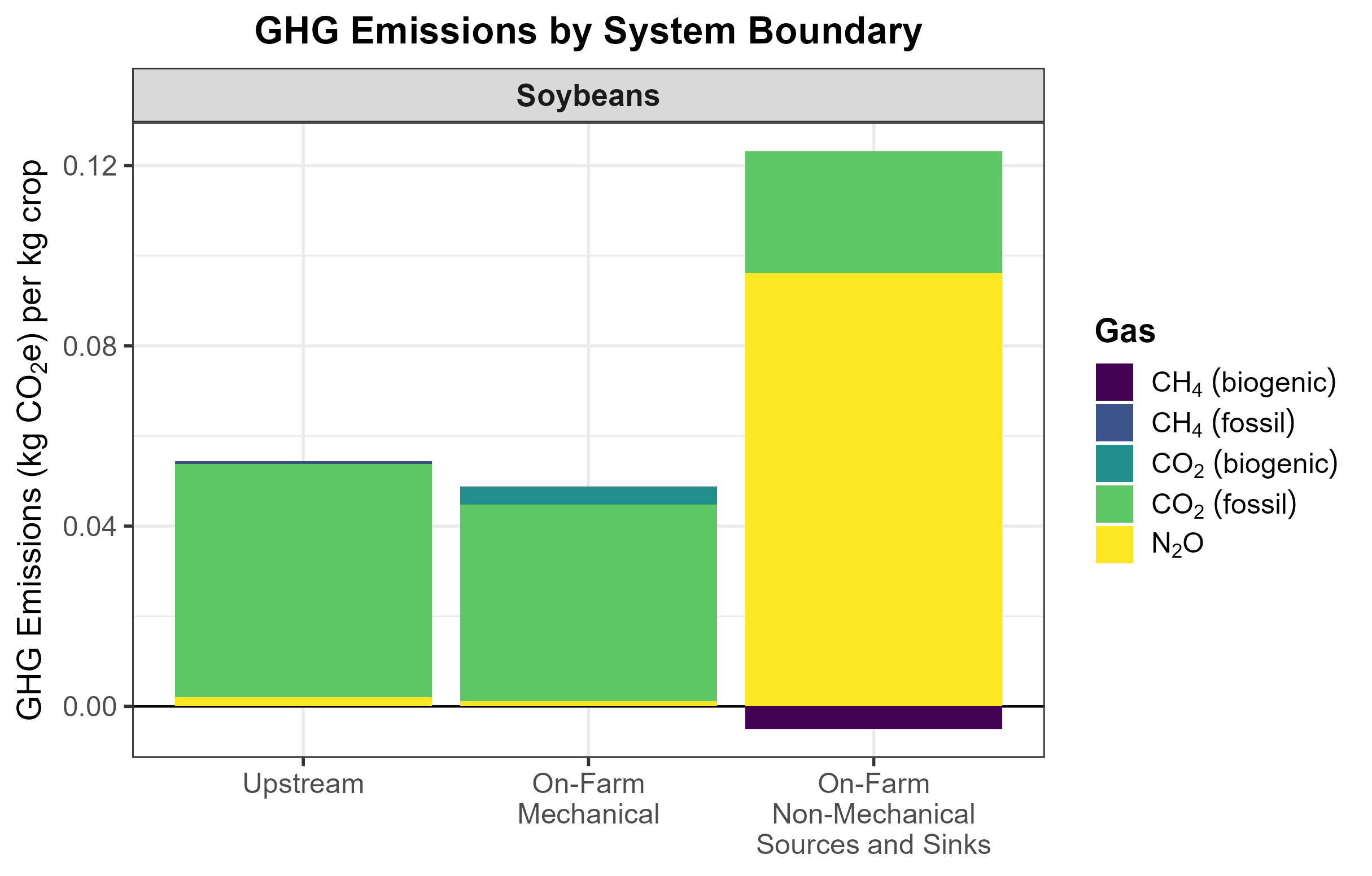
10.3 Winter wheat
- Location: Hodgeman County, Kansas.
- Yield: 62 bushel/acre.
- Diesel used for field operations: 7 gallon/acre.
- N-P2O5-K2O rates: 101-30-25.
- Lime rate: 500 lb/acre.
- Rainfed.
- Transportation distance from the field to the farm grain drying system: 25 miles.
- Amount of moisture removed through drying: 3%.
- Seeding rate of 157 lb/acre or approximately 1,500,000 seeds/acre.
- Approximately half the field was set on fire before planting to remove corn residue from the previous year.
- Pesticides: 3 herbicide products, 2 insecticide products, 2 fungicide products, 1 growth regulator, treated seed.
10.3.1 Results
- The aggregated estimate is 0.59 kg CO2e/kg wheat.
- Disaggregated estimates are shown in Figure 11.
- 57% of GHG emissions are coming from soil N2O.
- Area-based emissions are 2,461 kg CO2e/hectare. Considering the small amount of estimated biogenic CH4 being sequestered, net emissions are 2,439 kg CO2e/hectare.
- Setting crop residue on fire for half the field contributed 230 kg CO2e/hectare.
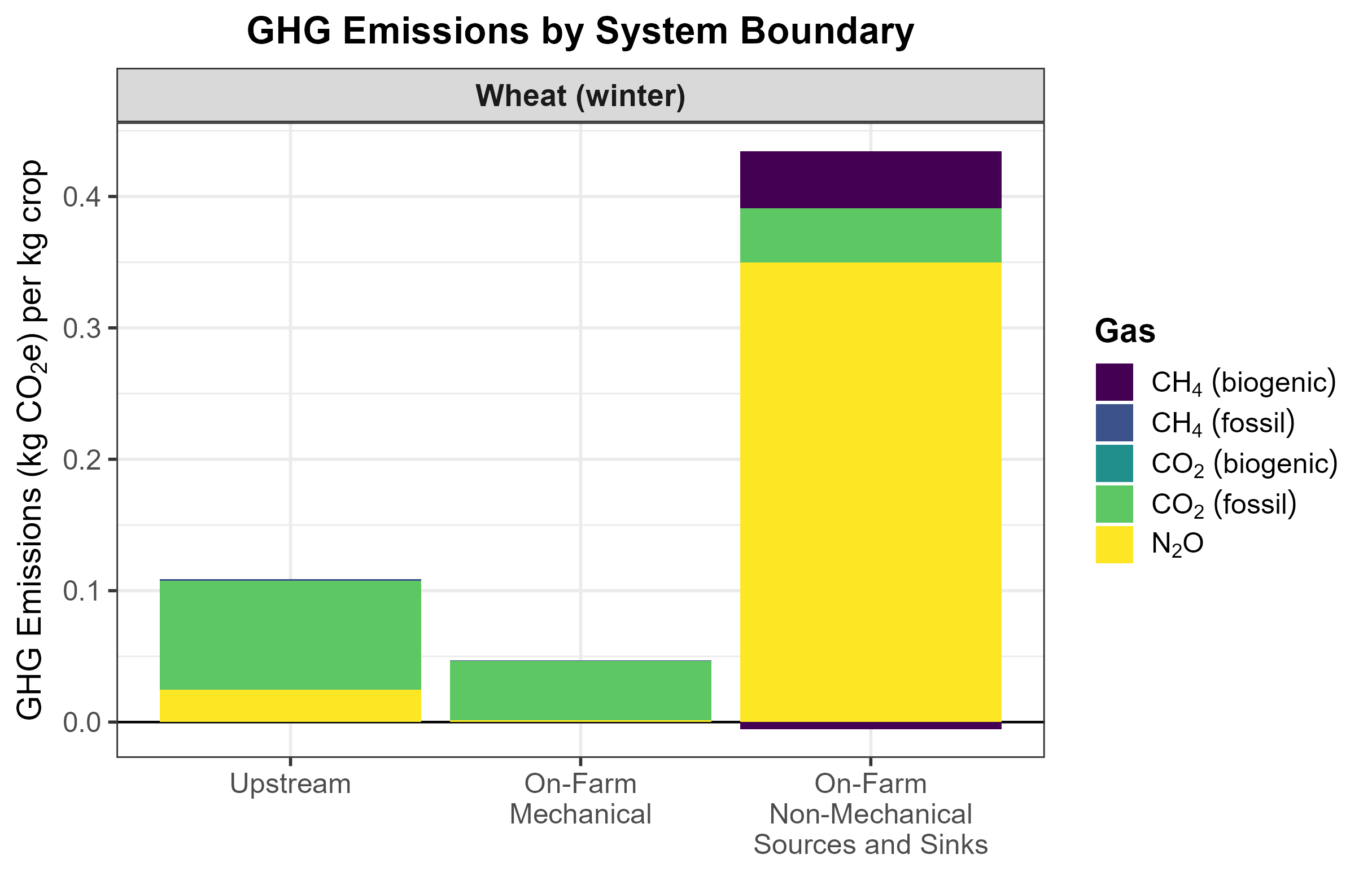
10.4 Cotton
10.4.1 Production inputs
- Location: Tift County, Georgia.
- Yield: 1,200 lb/acre of lint.
- Diesel used for field operations: 9 gallon/acre.
- N-P2O5-K2O rates: 90-70-70; no use of slow-release N fertilizers or N inhibitors.
- Lime rate: 660 lb/acre.
- Irrigation rate of 13 acre-inches/acre; well depth of 250 ft; pump pressure of 50 psi; pump powered by electricity.
- Transportation distance from the field to the ginning facility: 25 miles.
- Cotton lint wetter than normal.
- Seeding rate of 19 lb/acre or approximately 85,000 seeds/acre.
- Pesticides: 3 herbicide products, 2 insecticide products, 2 fungicide products, 2 growth regulators, treated seed.
10.4.2 Results
- The aggregated estimate is 2.21 kg CO2e/kg cotton output (lint and seed). Considering the 83% allocation to lint, the final estimate is 1.8 kg CO2e/kg cotton lint.
- Disaggregated estimates are shown in Figure 12.
- 36% of GHG emissions are coming from soil N2O.
- Area-based emissions are 2,804 kg CO2e/hectare for production of lint and seed. Considering the small amount of estimated biogenic CH4 being sequestered, net emissions are 2,780 kg CO2e/hectare, or 2,307 kg CO2e/hectare allocated to the lint.
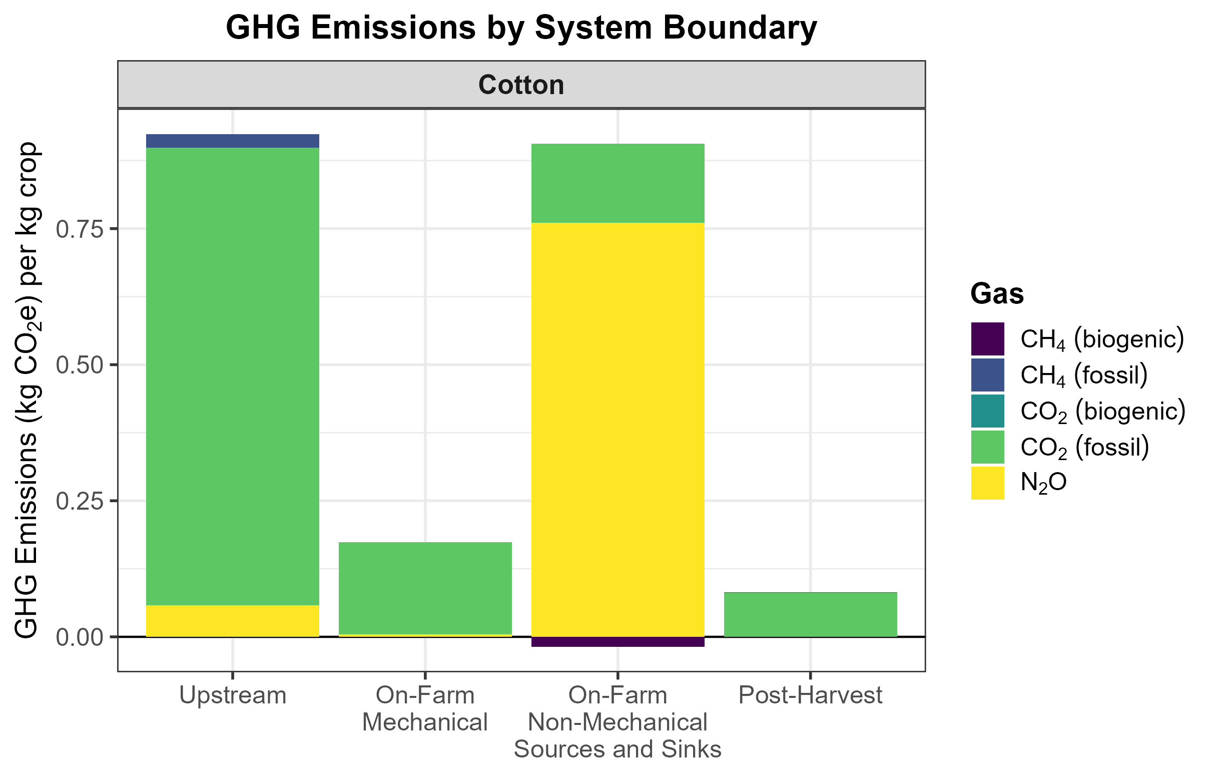
10.5 Peanuts
10.5.1 Production inputs
- Location: Tift County, Georgia.
- Yield: 4,700 lb/acre.
- Diesel used for field operations: 12 gallon/acre.
- No N-P2O5-K2O needed; 1 application of micronutrients (boron).
- Gypsum rate: 1,000 lb/acre.
- Irrigation rate of 8 acre-inches/acre; well depth of 250 ft; pump pressure of 50 psi; pump powered by diesel.
- Transportation distance from the field to the peanut buying point: 15 miles.
- Amount of moisture removed through drying: 7%.
- Seeding rate of 130 lb/acre or approximately 59,800 seeds/acre.
- Pesticides: 3 herbicide products, 2 insecticide products, 6 fungicide products, inoculant, treated seed.
10.5.2 Results
- The aggregated estimate is 0.47 kg CO2e/kg peanuts.
- Disaggregated estimates are shown in Figure 13.
- 39% of GHG emissions are coming from soil N2O. Although there were no applications of N fertilizer, the soil N2O model considers crop residue as another input that can result in a release of N2O emissions.
- Area-based emissions are 2,492 kg CO2e/hectare. Considering the small amount of estimated biogenic CH4 being sequestered, net emissions are 2,469 kg CO2e/hectare.
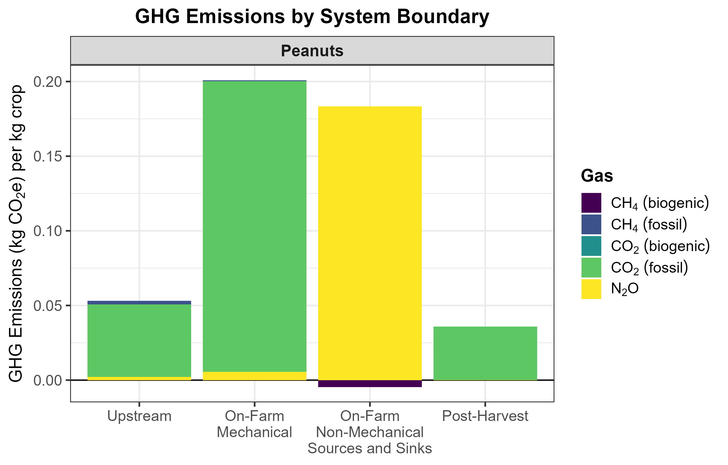
10.6 Chickpeas (garbanzos)
10.6.1 Production inputs
- Location: Fallon County, Montana.
- Yield: 1,574 lb/acre.
- Diesel used for field operations: 6 gallon/acre.
- N-P2O5-K2O rates: 10-25-10; no use of slow-release N fertilizers or N inhibitors.
- Rainfed.
- Transportation distance from the field to the processing facility: 45 miles.
- Crop does not need to be dried.
- Seeding rate of 159 lb/acre.
- Pesticides: 2 herbicide products, 2 insecticide product, 1 fungicide product, inoculant, treated seed.
10.6.2 Results
- The aggregated estimate is 0.3 kg CO2e/kg chickpeas.
- Disaggregated estimates are shown in Figure 14.
- 37% of GHG emissions are coming from soil N2O.
- Area-based emissions are 527 kg CO2e/hectare. Considering the small amount of estimated biogenic CH4 being sequestered, net emissions are 505 kg CO2e/hectare.
.png)
10.7 Potatoes
10.7.1 Production inputs
- Location: Bingham County, Idaho.
- Yield: 420 cwt/acre.
- Diesel used for field operations: 24 gallon/acre.
- N-P2O5-K2O-S rates: 260-235-215-85; no use of slow-release N fertilizers or N inhibitors.
- Irrigation rate of 21 acre-inches/acre; well depth of 500 ft; pump pressure of 250 psi; pump powered by electricity.
- Transportation distance from the field to the farm storage system: 5 miles.
- Seeding rate of 6,965 lb/acre or approximately 34,800 seeds/acre.
- Pesticides: 4 herbicide products, 4 insecticide products, 3 fungicide products, 1 growth regulator, 1 fumigant, 1 application of sulfuric acid, treated seed.
10.7.2 Results
- The aggregated estimate is 0.15 kg CO2e/kg potatoes.
- Disaggregated estimates are shown in Figure 15.
- 38% of GHG emissions are coming from soil N2O.
- Area-based emissions are 7,176 kg CO2e/hectare. Considering the small amount of estimated biogenic CH4 being sequestered, net emissions are 7,152 kg CO2e/hectare.
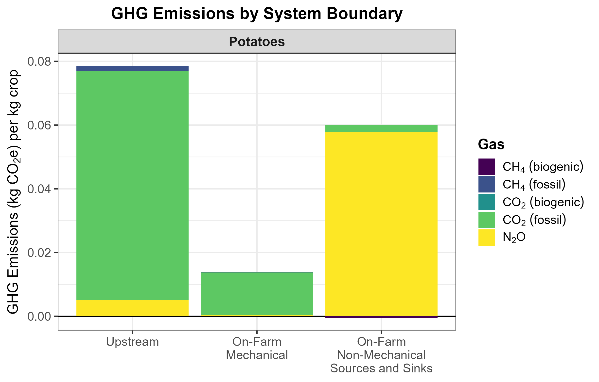
10.8 Sorghum
10.8.1 Production inputs
- Location: Hodgeman County, Kansas.
- Yield: 66 bushel/acre.
- Diesel used for field operations: 6 gallon/acre.
- N-P2O5-K2O rates: 140-60-15; no use of slow-release N fertilizers or N inhibitors.
- Irrigation rate of 15 acre-inches/acre; well depth of 150 ft; pump pressure of 75 psi; pump powered by electricity.
- Transportation distance from the field to the storage facility: 15 miles.
- Crop does not need to be dried.
- Seeding rate of 12 lb/acre or approximately 100,000 seeds/acre.
- Pesticides: 2 herbicide products, 1 insecticide product, 1 fungicide product, treated seed.
10.8.2 Results
- The aggregated estimate is 0.73 kg CO2e/kg sorghum.
- Disaggregated estimates are shown in Figure 16.
- 55% of GHG emissions are coming from soil N2O.
- Area-based emissions are 3,009 kg CO2e/hectare. Considering the small amount of estimated biogenic CH4 being sequestered, net emissions are 2,987 kg CO2e/hectare.
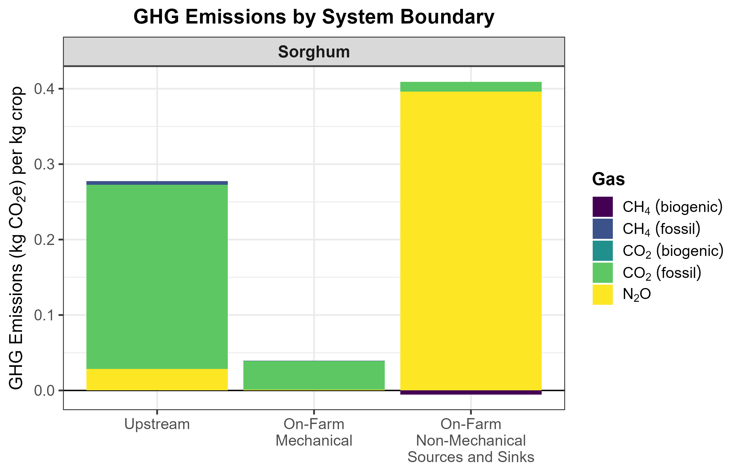
10.9 Sugar beets
10.9.1 Production inputs
- Location: Crook County, Oregon.
- Yield: 22 ton/acre with 18% sugar content (2,000 lb/ton).
- Diesel used for field operations: 14 gallon/acre.
- N-P2O5-K2O rates: 106-148-46; no use of slow-release N fertilizers or N inhibitors.
- Lime rate of 500 lb/acre.
- Irrigation rate of 25 acre-inches/acre; well depth of 250 ft; pump pressure of 50 psi; pump powered by electricity.
- Transportation distance from the field to the farm storage system: 25 miles.
- Seeding rate of 20 lb/acre.
- Pesticides: 2 herbicide products, 1 insecticide product, 4 fungicide products, 1 growth regulator, 1 fumigant, treated seed.
10.9.2 Results
- The aggregated estimate is 0.57 kg CO2e/kg sugar.
- Disaggregated estimates are shown in Figure 17.
- 57% of GHG emissions are coming from soil N2O.
- Area-based emissions are 5,093 kg CO2e/hectare. Considering the small amount of estimated biogenic CH4 being sequestered, net emissions are 5,068 kg CO2e/hectare.
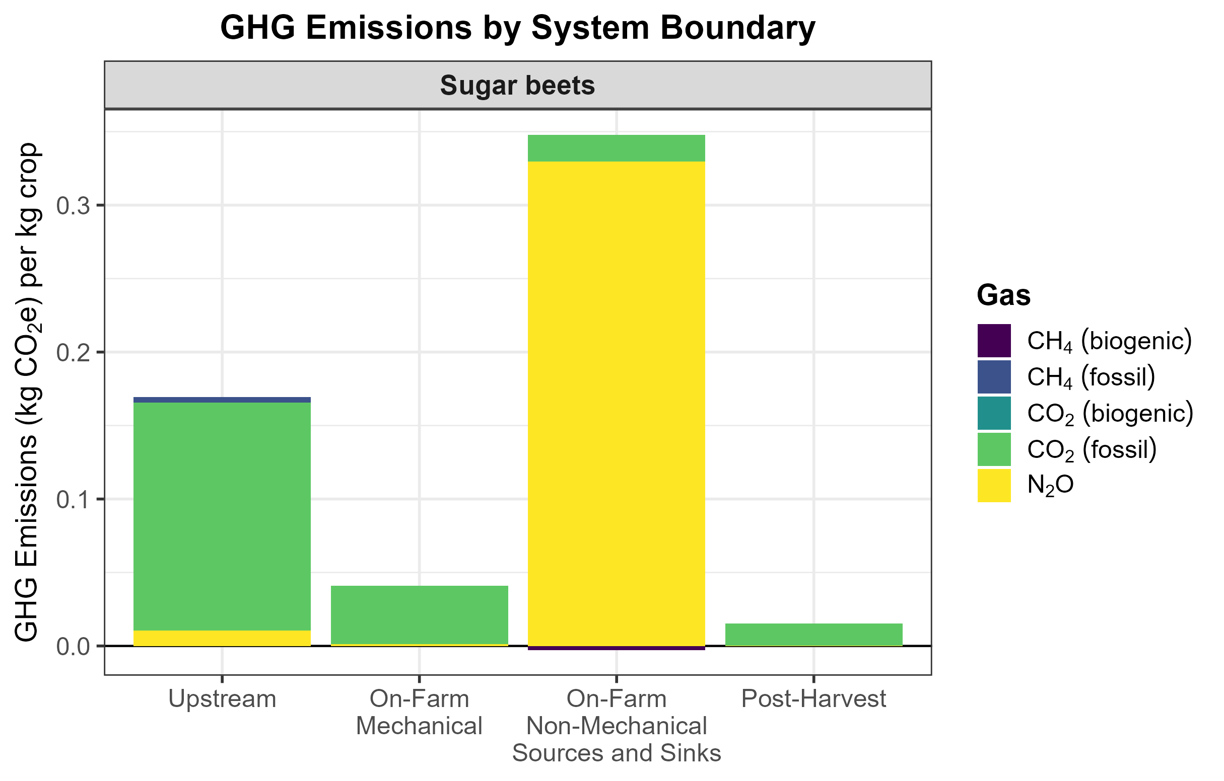
10.10 Rice (Mid-South)
10.10.1 Production inputs
- Location: Monroe County, Arkansas.
- Yield: 74 cwt/acre.
- Diesel used for field operations: 8 gallon/acre.
- N-P2O5-K2O rates: 170-93-46; no use of slow-release N fertilizers or N inhibitors.
- Lime rate: 500 lb/acre.
- Irrigation rate of 30 acre-inches/acre; well depth of 50 ft; pump pressure of 50 psi; pump powered by electricity.
- Transportation distance from the field to the storage facility: 25 miles.
- Amount of moisture removed: 3%.
- Water management: continuously flooded.
- Soil clay content: 23%.
- Non-flooded pre-season.
- Planting into low residue; drill seeded.
- Seeding rate of 156 lb/acre.
- Pesticides: 2 herbicide products, 2 insecticide products, 1 fungicide product, treated seed.
10.10.2 Results
- The aggregated estimate is 1.18 kg CO2e/kg rice.
- Disaggregated estimates are shown in Figure 18.
- 65% of GHG emissions are coming from CH4.
- Area-based emissions are 9,262 kg CO2e/hectare.
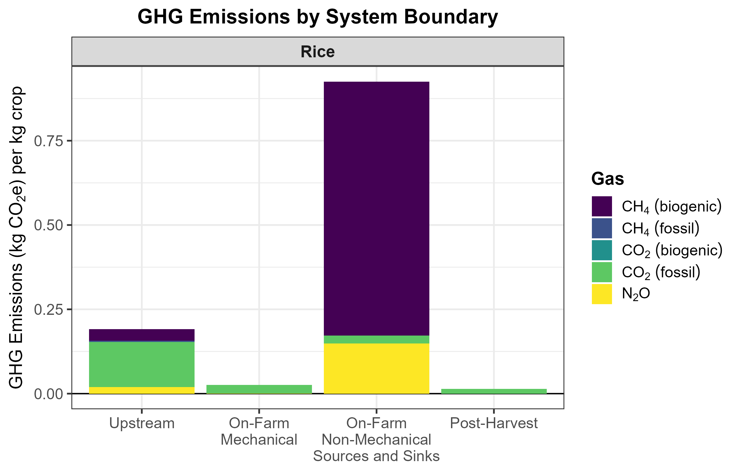
10.11 Rice (California)
10.11.1 Production inputs
- Location: Colusa County, California.
- Yield: 85 cwt/acre.
- Diesel used for field operations: 8 gallon/acre.
- N-P2O5-K2O rates: 170-93-46; no use of slow-release N fertilizers or N inhibitors.
- Lime rate: 500 lb/acre.
- Irrigation rate of 30 acre-inches/acre; well depth of 50 ft; pump pressure of 50 psi; pump powered by electricity.
- Transportation distance from the field to the storage facility: 25 miles.
- Amount of moisture removed: 3%.
- Water management: continuously flooded.
- Soil clay content: 46%.
- Flooded pre-season > 30 days.
- Planting into high residue; water seeded.
- Seeding rate of 156 lb/acre.
- Pesticides: 2 herbicide products, 2 insecticide products, 1 fungicide product, treated seed.
10.11.2 Results
- The aggregated estimate is 1.06 kg CO2e/kg rice.
- Disaggregated estimates are shown in Figure 19.
- 66% of GHG emissions are coming from CH4.
- Area-based emissions are 9,713 kg CO2e/hectare.
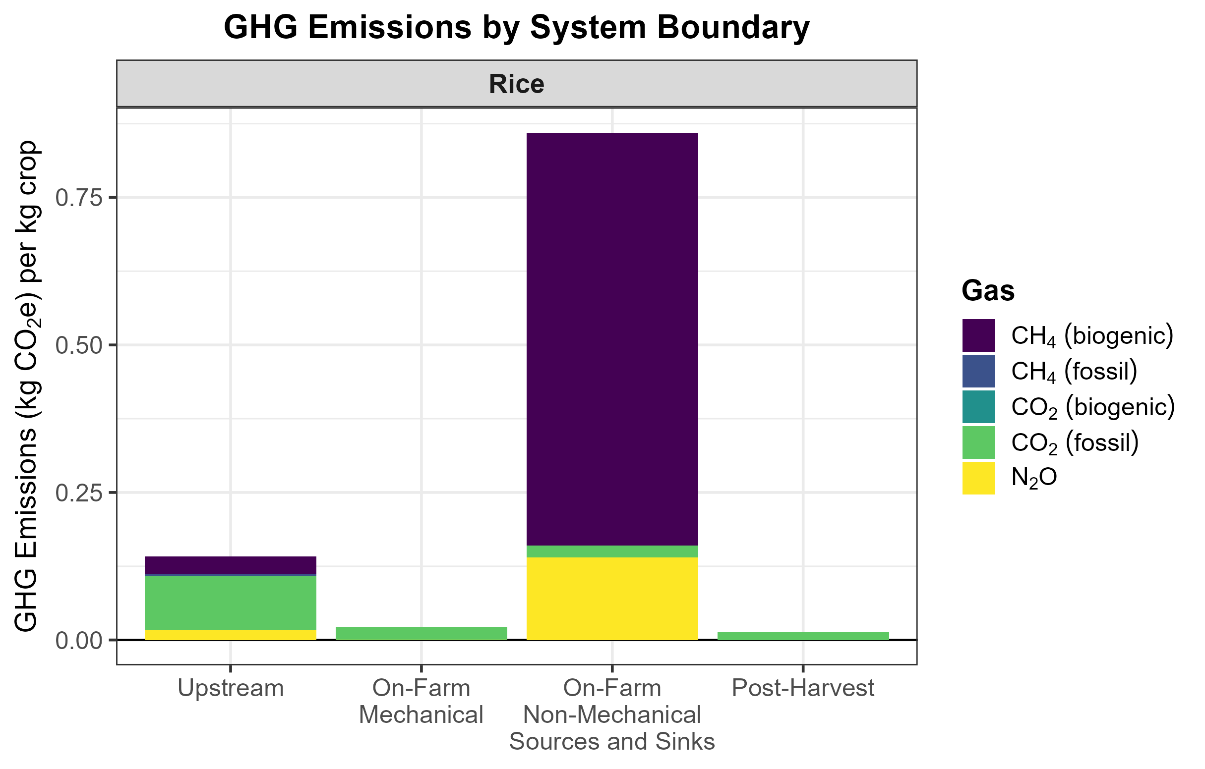
References
Arkansas. 2024. Pumping Plant Efficiency. https://www.uaex.uada.edu/environment-nature/water/agriculture-irrigation/pumping-plant-efficiency.aspx.
Audsley, Eric, K Stacey, DJ Parsons, and AG Williams. 2009. Estimation of the Greenhouse Gas Emissions from Agricultural Pesticide Manufacture and Use. https://doi.org/10.13140/RG.2.1.5095.3122.
Bigelow, Daniel. 2014. USDA Economic Research Service-Farmland Ownership and Tenure. https://www.ers.usda.gov/topics/farm-economy/land-use-land-value-tenure/farmland-ownership-and-tenure.
BLS. 2017. Commodity Flow Survey (CFS). Bureau of Transportation Statistics. https://www.bts.gov/cfs.
Boryan, Claire, Zhengwei Yang, Rick Mueller, and Mike Craig. 2011. “Monitoring US Agriculture: The US Department of Agriculture, National Agricultural Statistics Service, Cropland Data Layer Program.” Geocarto International 26 (5): 341–58.
EC–European Commission. 2010. “2010/335/: Commission Decision of 10 June 2010 on Guidelines for the Calculation of Land Carbon Stocks for the Purpose of Annex v to Directive 2009/28/EC (Notified Under Document c(2010) 3751).” In Official Journal of the European Union. https://eur-lex.europa.eu/eli/dec/2010/335/oj.
Eisenhauer, Dean E, Derrel L Martin, Derek M Heeren, and Glenn J Hoffman. 2021. Irrigation Systems Management. American Society of Agricultural; Biological Engineers (ASABE).
Fipps, Guy. 1995. Calculating Horsepower Requirements and Sizing Irrigation Supply Pipelines.
Green, MR. 1987. “Energy in Pesticide Manufacture, Distribution and Use.” Energy in Plant Nutrition and Pest Control.
Harrison, Kerry. 2012. Irrigation Pumping Plants and Energy Use. https://extension.uga.edu/publications/detail.html?number=B837&title=irrigation-pumping-plants-and-energy-use.
Hoffman, Glenn J, TA Howell, and Kenneth H Solomon. 1990. Management of Farm Irrigation Systems. American Society of Agricultural Engineers.
IPCC. 2019. “2019 Refinement to the 2006 IPCC Guidelines for National Greenhouse Gas Inventories.” In Agriculture, Forestry and Other Land Use, vol. 4. IPCC Geneva, Switzerland:
Kottek, Markus, Jürgen Grieser, Christoph Beck, Bruno Rudolf, and Franz Rubel. 2006. “World Map of the Köppen-Geiger Climate Classification Updated.” Meteorologische Zeitschrift 15 (3): 259–63. https://doi.org/10.1127/0941-2948/2006/0130.
Kucera, Michael J., and Christopher B. Coreil. 2023. “Overview of USDA-NRCS Erosion Prediction Technology and Conservation Resources - Land Management Operations Database and Use.” Soil Erosion Research Under a Changing Climate, January 8-13, 2023, Aguadilla, Puerto Rico, USA, ahead of print. https://doi.org/10.13031/soil.23007.
Liu, Xinyu, Hao Cai, Hoyoung Kwon, and Michael Wang. 2023. Feedstock Carbon Intensity Calculator (Fd-Cic): Users’ Manual and Technical Documentation. Argonne National Laboratory (ANL), Argonne, IL (United States).
Martin, Derrel L, Tom W Dorn, Steve R Melvin, Alan J Corr, and William Kranz. 2011. “Evaluating Energy Use for Pumping Irrigation Water.” February 22.
Ogle, Stephen M, Paul R Adler, Gary Bentrup, et al. 2024. “Chapter 3: Quantifying Greenhouse Gas Sources and Sinks in Cropland and Grazing Land Systems.” In: Hanson, Wes L.; Itle, Cortney; Edquist, Kara, Eds. Quantifying Greenhouse Gas Fluxes in Agriculture and Forestry: Methods for Entity-Scale Inventory. Technical Bulletin Number 1939, 2nd Edition. Washington, DC: US Department of Agriculture, Office of the Chief Economist. 6-1-6-23. Chapter 3. 1939: 3–1.
USDA-NRCS. n.d. USDA-NRCS Energy Consumption Awareness Tool: Irrigation. https://ipat.sc.egov.usda.gov/.