Proposing Revisions to the Energy Use, GHG Emissions, and Soil Carbon Metrics

Glossary

• International System of Units: Universally abbreviated SI (from the French Le Système International d’Unités), is the modern metric system of measurement (Newell, Tiesinga, et al. 2019). This includes units such as kilogram (kg) for mass, meter (m) for distance, and hectare (ha) for area. It will be referred to as SI units in this document.
• United States Customary System: System of units common in the United States. This includes units such as bushel for volume, lb (pound) for weight, mile for distance, and acre for area. It will be referred to as USCS units in this document.
• Fieldprint Platform: The Platform includes the Fieldprint Calculator and the Fieldprint Application Programming Interface (API), which serves corporations integrating Field to Market metrics into their software platforms.
• Fieldprint Analysis: The output or result from running the Fieldprint Platform for a given crop and year to obtain the metric scores.
• Hydrologic Unit Codes: Abbreviated as HUC, they represent geographic delineations of watersheds. HUCs range from HUC-2 (regions) to HUC-12 (sub-watersheds).

Abbreviations

• FP, Fieldprint Platform, including the Fieldprint Calculator and the Application Programming Interface (API) used by our Qualified Data Management Partners.
• FP v4.2, Fieldprint Platform version 4.2 (the current version to revise)
• FP v5, Fieldprint Platform version 5 (the version to implement)
• FTM, Field to Market
• GHG, greenhouse gas
• USDA, United States Department of Agriculture
• USEPA, United States Environmental Protection Agency
• IPCC, Intergovernmental Panel On Climate Change
• GWP, global warming potential
• HUC, Hydrologic Unit Codes
• HRU, Hydrologic Response Units

1 Purpose of this document

This document focuses on the revisions to three connected metrics: Energy Use, GHG Emissions, and Soil Carbon metrics. These three metrics are core to Field to Market’s programs.

We aim to provide sufficient detail to understand the upcoming changes. The revisions proposed here represent significant progress to align with well-accepted GHG emission quantification methods and achieve a superior level of rigor and transparency.

This major revision of the Fieldprint Platform will result in a version change. The current version is Fieldprint Platform version 4.2 (FP v4.2), and starting in mid-2025, it will be Fieldprint Platform version 5 (FP v5).

This document contains technical information. The language used here will, at times, be repetitive to reduce ambiguity.

2 Background

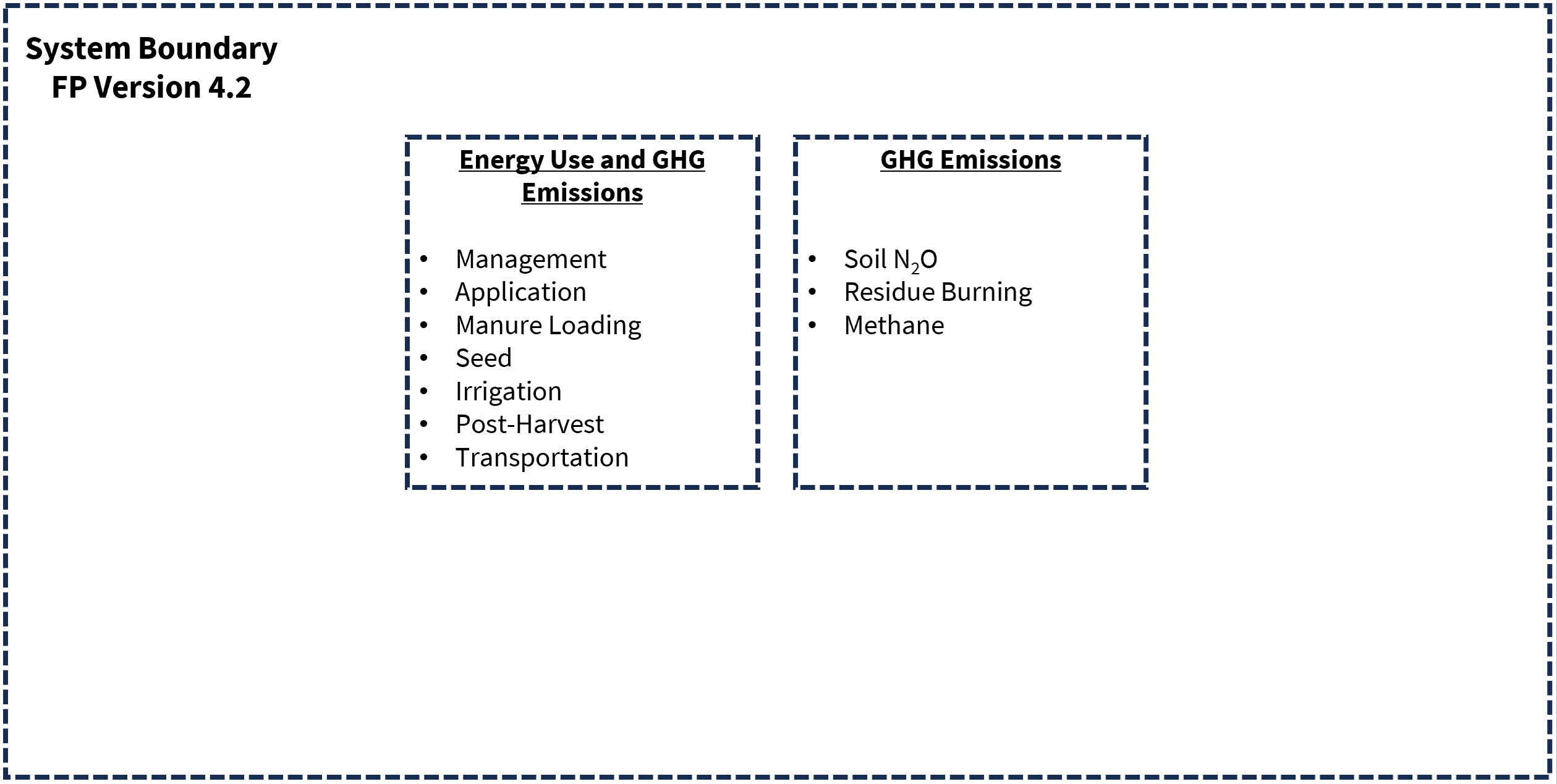
Field to Market last revised the Energy Use and GHG Emissions metrics in 2018 by updating the data sources, such as emission factors, while leaving the energy use and emission categories unchanged. The current Energy Use and GHG Emissions categories (Figure 1) have largely been based on Field to Market’s late-2000s work.

GHG emission quantification for agricultural production has advanced in rigor and standardization over the past fifteen years, and it is time for Field to Market to revise the metrics to align with life cycle analysis (LCA) principles and provide complete transparency about each energy use and GHG emission source. To complete the revision being proposed, we sought to update reference data and reorganize, revise, and add sources of GHG emissions to improve the usability of the FP and align with major standards.

Important

What is a life cycle analysis (LCA)?

From ISO (2006):

LCA is the compilation and evaluation of the inputs and outputs and the potential environmental impacts of a product system throughout its life cycle.

What is the use of LCA?

From Sieverding et al. (2020):

Life cycle analysis is used to quantify the environmental performance of products, processes, or services, and is increasingly being used as a basis to inform purchasers along the supply chain, including the end users (Fava, Baer, and Cooper 2011).

Field to Market staff has had many interactions with growers and stakeholders over the years, and several of the proposed changes reflect the feedback we have received about improving the usability of the FP.

The FP is built on a bespoke analytical engine; reference data, algorithms, and models are coded for the calculations feeding into the metrics. Over the years, and particularly with the proposed revisions, the FP engine has increased in complexity. To provide transparency, Field to Market plans to release a metric documentation website for the suite of sustainability metrics in mid-2025 and publish a journal article at a later date.

3 Scope of the revisions

From its origins, Field to Market developed the Fieldprint Platform as a streamlined LCA tool to estimate the environmental impact of row crop production. The revisions proposed here strengthen the Fieldprint Platform’s original objective. We aim to provide a tool that is robust, transparent, and reproducible.

The objectives of this revision were to complete the following fourteen tasks:

1. Clarify the system boundary and reorganize the energy use and GHG emission sources to enable disaggregation. The system boundary is a definition of what is included or excluded from the analysis (Czyrnek-Delêtre, Smyth, and Murphy 2017). Disaggregation is needed to better understand sources of GHG emissions and to align with major standards (see Supplementary Material for more information on disaggregation).
2. Update the default global warming potential (GWP) factors and include additional GWP factors as a user or project option.
3. Update energy use and GHG emission impact factors, including factors for electricity, fuels, fertilizers, pesticides, and seeds.
4. Revise fertilizer, pesticide, and organic amendment options, and add new ones.
5. Update the pesticide rate assumptions for each crop.
6. Include gas separation for sources of GHG emissions, focusing on CO₂ (biogenic and fossil), CH₄ (biogenic and fossil), and N₂O. Electricity factors also include estimates for NF3 and SF6.
7. Include upstream energy use and associated GHG emissions from electricity generation and distribution and fuel manufacturing.
8. Review and update algorithms used to estimate energy use and associated GHG emissions from the following activities:
   • Irrigation operations
   • Field operations
   • Manure transportation
   • Crop transportation
   • Crop drying
9. Account for cover cropping activities.
10. Enable accounting for more than one cash crop per calendar year (e.g. double-cropping), fallow years, and crop failures.
11. Streamline algorithms and the user interface by removing rarely-used options and pre-filling inputs of minimal impact. Pre-filled inputs can be edited by users.
12. Update three GHG emission methods using the 2024 USDA publication of methods for entity-scale inventory (Ogle et al. 2024):
    • Soil N₂O (direct and indirect)
    • Non-CO₂ emissions from biomass burning
    • CH₄ emissions from flooded rice cultivation
13. Add four GHG emission quantification methods from the 2024 USDA publication of methods for entity-scale inventory (Ogle et al. 2024) and Intergovernmental Panel on Climate Change (IPCC 2019):
    • CH₄ flux from non-flooded soils
    • CO₂ from carbonate lime applications to soils
    • CO₂ from urea fertilizer applications
    • Direct land use change
14. Implement SWAT+ (Soil and Water Assessment Tool Plus) to quantify soil carbon stock change. SWAT+ is a Tier 3 model. See Important 1 for more information about Tiers.

4 Timeline of relevant activities

• 2009
  • Energy Use and GHG Emissions are included as metrics in Field to Market’s programs.
• 2012
  • Soil Carbon is included as a metric in Field to Market’s programs. The Soil Conditioning Index (USDA 2003) is selected as the model of choice. Colorado State University starts providing Soil Conditioning Index modeling results as part of their suite of model services (Carlson 2016).
• 2017-2018
  • Impact factors, algorithms, and reference data for Energy Use and GHG Emissions metrics are updated for the 2018 release of the Fieldprint Platform. Addition of rice methane and soil N₂O modules.
• 2016-2021
  • Field to Market explores several times the possibility of upgrading the model of choice for the Soil Carbon metric to use a quantitative model rather than an index. Many efforts do not progress due to data requirements and inadequate digital infrastructure. In 2021, Field to Market adds COMET-Planner (Field to Market 2021; Swan et al. 2018) as an easy-to-use tool to estimate GHG emission reductions for practice change scenarios in croplands.
• 2023
  • In collaboration with several organizations, Field to Market explores the possibility of a multi-model ensemble for soil carbon modeling. While the multi-model ensemble effort does not progress, Colorado State University One Water Solutions Institute announces plans to add SWAT+ to the suite of modeling service offerings.
  • While preparing for a third-party review, Field to Market staff conducts a comprehensive internal review and determines that a revision to Energy Use and GHG Emissions metrics is warranted. The Metrics Committee agrees to pursue the revision, and forms a Sub-Committee to tackle the detailed work. The Sub-Committee meets several times to develop an updated framework for Energy Use and GHG Emissions.
• 2024
  • Field to Market iterates improvements with the Metrics Committee after requesting and receiving feedback from several experts in the LCA and GHG emission quantification space. Field to Market hires an external consultant to assist with the revisions. Concurrently, Field to Market staff updates the methodology for estimating energy use and associated GHG emissions from irrigation operations, manure transport, crop drying, field operations, and crop transport.
• 2025 (current activity)
  • Field to Market proposes metric revisions to members.

5 Introducing Fieldprint Platform Version 5 with revisions to Energy Use, GHG Emissions, and Soil Carbon metrics

The agricultural sector represents approximately 10% of the total greenhouse gas (GHG) emissions in the United States (USEPA 2023b) and has been recognized as a significant contributor to water quality impairment (Shortle, Abler, and Ribaudo 2001), water depletion (Rosa et al. 2020), biodiversity loss (Kehoe et al. 2017), and soil degradation (Thaler, Larsen, and Yu 2021). Of course, agricultural production is key to stable societies, and agricultural landscapes are part of the ecosystems providing critical services such as drinking water, waste decomposition, carbon storage, and support of aquatic, terrestrial, microbial, and below-ground species (Tilman and Clark 2015).

Stakeholders in the agricultural value chain, from growers to manufacturers, processors, and retailers, are strongly interested in identifying the key contributors to environmental impact and finding solutions to reduce those impacts at scale.

It is critical for the agricultural industry in the United States to have a transparent, accessible, and stable method to measure their impact yearly. This enables the agricultural value chain to analyze progress, quantify the impact of alternative production scenarios, and report sustainability outcomes. The Fieldprint Platform was designed for those purposes. Field to Market firmly believes that the tools and models to measure and improve crop production sustainability should be available to all stakeholders in the agricultural sector.

5.1 Proposed goal and scope of FP v5

The primary goal of the Fieldprint Platform is to evaluate the environmental impact associated with the agricultural production of twenty row crop commodities (Table 1) at the field level. The outcomes from individual fields can be aggregated to represent a farm or a supply shed (a group of farmer suppliers in a defined geography or market). Considering all 2024 planted acres (harvested acres for alfalfa) of crops in Field to Market’s program, the Fieldprint Platform can be used to quantify the impact of approximately 267 million acres (108 million hectares) of United States cropland, representing nearly 70% (267M/382M) of all U.S. planted cropland (USDA NASS 2024a).

Table 1: Crops included in the Fieldprint Platform

Crop	Crop Production Unit (SI Units)	Crop Production Unit (USCS Units)	lb / unit (USCS Units)	Production Output
Alfalfa	kg	ton	2,000	Forage or Biomass
Barley	kg	bushel	48	Grain or seed
Chickpeas (garbanzos)	kg	lb	1	Grain or seed
Corn (grain)	kg	bushel	56	Grain or seed
Corn (silage)	kg	ton	2,000	Forage or Biomass
Cotton	kg	lb	1	Lint
Dry Beans	kg	lb	1	Grain or seed
Dry Peas	kg	lb	1	Grain or seed
Fava Beans	kg	lb	1	Grain or seed
Lentils	kg	lb	1	Grain or seed
Lupin	kg	lb	1	Grain or seed
Peanuts	kg	lb	1	Grain or seed
Potatoes	kg	cwt	100	Tuber
Rice	kg	cwt	100	Grain or seed
Sorghum	kg	bushel	56	Grain or seed
Soybeans	kg	bushel	60	Grain or seed
Sugar beets	kg	ton sugar	2,000	Root
Wheat (durum)	kg	bushel	60	Grain or seed
Wheat (spring)	kg	bushel	60	Grain or seed
Wheat (winter)	kg	bushel	60	Grain or seed

For the three metrics being revised, the impacts are defined as follows:

• The Energy Use metric estimates the cumulative energy demand (CED) associated with producing a given crop. The CED accounts for the primary energy, from fossil and non-fossil sources, used throughout the life cycle, including upstream supply chains.
• The GHG Emissions metric estimates emissions associated with producing a given crop. The estimated gases are converted to Global Warming Potential (GWP) using 100-yr time horizon factors from the Intergovernmental Panel on Climate Change Sixth Assessment Report (AR6) (Pier et al. 2021). While the AR6 100-yr factors will be the default, Fieldprint Platform users will have the ability to choose other GWP factors. The list of GWP factors is posted here.
• The Soil Carbon metric estimates annual soil carbon stock changes from consecutive calendar years (e.g. December 31, 2023 to December 31, 2024) for a given field boundary, using crop rotation and management history from 2008 to the latest available growing season.

The proposed SI units and USCS units for the three metrics being revised are shown in Table 2.

Table 2: Proposed units for the metrics being revised for Fieldprint Platform Version 5

Metric	SI Units	USCS Units
Energy Use	MJ / kg crop	BTU / crop production unit
Greenhouse Gas Emissions	kg CO2e / kg crop	lb CO2e / crop production unit
Soil Carbon	Δ kg CO2 / ha / year	Δ lb CO2 / acre / year

The Fieldprint Platform is designed to produce an attributional, streamlined life cycle analysis of a given crop. Attributional LCAs are common in agriculture (Sieverding et al. 2020); the analysis is detailed and process-specific, which enables growers and organizations in the agricultural value chain to evaluate the environmental outcomes of business-as-usual practices, compare them with potential improvement scenarios, and find ways to incentivize practices for which there is evidence of a reduced environmental impact.

Streamlined LCA, as opposed to a traditional or full LCA, is a resource-efficient method to identify key contributors to GHG emissions, among other impacts (Pelton 2018; Verghese, Horne, and Carre 2010). Streamlined LCAs focus on limited impact categories and reduce the barriers to conducting assessments of the environmental impact of crop production (Pelton 2018). Agriculture is one of many industries utilizing streamlined LCA to detect the highest contributors of GHG emissions and other environmental impacts. The literature contains many examples of streamlined LCA from the automotive (Arena, Azzone, and Conte 2013), packaging (Verghese, Horne, and Carre 2010), solid waste management (Y. Wang, Levis, and Barlaz 2021), and construction (Heidari et al. 2019) industries.

The simplification of LCA could result in too many shortcuts and assumptions that jeopardize their accuracy and utility (Verghese, Horne, and Carre 2010; Hunt et al. 1998). The Fieldprint Platform’s streamlined LCA model aims to achieve an acceptable balance between the practicality and completeness of the analysis (see Section 5.4.2.2 for excluded sources, Section 5.6 for data inputs, and Section 10 for other known limitations). Since the crops in Field to Market’s program produce grain, seeds, harvestable tubers and roots, and forage or biomass on an annual basis, the Fieldprint Platform represents an accessible and stable method to support agricultural industry stakeholders in their efforts to measure and reduce the environmental impact of crop production.

5.2 How does the Fieldprint Platform work?

GHG emissions from agricultural activities are typically quantified in three primary ways:

1. Direct measurements, including soil sampling for soil carbon stock changes (Wendt and Hauser 2013) or eddy-covariance measurements for GHG fluxes (Baldocchi et al. 2001).
2. Impact factors, which include energy or emission factors, such as those hosted by IPCC (2022) and other open and commercial sources.
3. Process-based models, where models simulate the impacts on GHG emissions by agricultural activities (Sándor et al. 2018; Zhang et al. 2013).

All methods have advantages and limitations (Bastviken et al. 2022). To address the limitations of the approaches described above, there are promising initiatives being applied to create system-of-systems, integrating modeling, ground observations and sensors, and computational techniques (Guan et al. 2023). These approaches might gain broad usage as transparency, reproducibility, and cost-effectiveness build confidence to replace standard approaches.

The FP v5 will estimate energy use and GHG emissions using impact factors, Tier 1 and Tier 2 approaches, and process-based models, which are considered a Tier 3 approach by IPCC (2019). Soil carbon stock changes will be estimated with a process-based model. The summary of approaches for the three metrics being revised is shown starting in Section 7.

Important 1

What are Tier 1, 2, and 3 approaches?

From the overview of IPCC (2019):

• Tier 1 represents the simplest methods, using default equations and emission factors provided in the IPCC guidance.
• Tier 2 uses default methods, but emission factors that are specific to different regions.
• Tier 3 uses country‐specific estimation methods, such as a process‐based model.

From the executive summary of Hanson et al. (2024):

GHG emission quantification approaches include multiple levels or tiers of complexity and accuracy, based on the best available data and methods.

The GHG emission methods published by Hanson et al. (2024) take a slightly modified approach from IPCC tiers, calling them instead Basic Estimation Equation, Inference, Modified IPCC or Empirical Model, and Processed‐Based Model. They are described as follows:

• Basic estimation equations use default equations and emission factors, such as IPCC Tier 1 methods.
• Inference uses geography‐, crop‐, livestock‐, technology‐, or practice‐specific emission factors to approximate emissions/removal factors. This approach is similar to an IPCC Tier 2 method and is more accurate, more complex, and requires more data inputs than the basic estimation.
• Modified IPCC/empirical and/or process‐based modeling, comparable to IPCC Tier 2 or IPCC Tier 3 methods. These methods are the most demanding in terms of complexity and data requirements and produce the most accurate estimates.

The FP v5 will work in the following manner:

• Growers draw a field boundary and enter the primary production data for that field based on their best knowledge and records (see Section 5.6 for a general description of grower inputs). The field boundary allows the FP to gather soil properties (soil type, texture, etc.), weather records, precipitation regimen, pre-fill the crop history sequence from 2008 to the latest available year, and select the electric grid. The field location also enables the FP to select the corresponding factors and reference data for several other models: CH₄ flux from non-flooded soils, direct land use change, soil N₂O, CH₄ emissions from flooded rice cultivation, and soil carbon stock changes.
• Based on the agricultural inputs applied (fertilizers, pesticides, seed), the quantities are multiplied by the corresponding impact factors.
• Based on the manure rate and type, the manure transportation method estimates the diesel fuel usage for loading and transportation. The amount of diesel is multiplied by the corresponding impact factors.
• If a field is irrigated, the irrigation operation method estimates the electricity or fuel usage to pump the gross amount of irrigation water pumped. The amount of electricity or fuel is multiplied by the corresponding impact factors.
• If a crop is mechanically dried to reach standard moisture, the crop drying method estimates the electricity and fuel usage required to dry the crop, based on the amount of moisture removed. The amount of electricity and fuel is multiplied by the corresponding impact factors.
• Based on the distance of the field to the drying, storage, or purchasing facility, the crop transportation method estimates the fuel usage to transport the crop production output. The amount of fuel is multiplied by the corresponding impact factors.
• Based on the field activities (plant, harvest, tillage, nutrient and pesticide applications, etc.), the field operations method uses the CRLMOD reference data (Kucera and Coreil 2023) to estimate the diesel fuel usage for the crop interval (crop intervals are explained here). The amount of fuel is multiplied by the corresponding impact factors.
• The crop rotation and management history, from 2008 to the latest available year, is sent to Colorado State University Cloud Services Integration Platform (David et al. 2014) to run the SWAT+ model to estimate soil carbon stock changes. Colorado State University also runs the models for the Soil Conservation and Water Quality metrics. The Soil Conservation and Water Quality metrics are not discussed at length in this document and they are not under revision.
• If a grower indicates that lime was applied, the CO₂ from carbonate lime applications to soils method is run.
• If a grower indicates that urea was applied, the CO₂ from urea fertilizer applications is run.
• If a grower indicates that crop residue was set on fire, the non-CO₂ emissions from biomass burning method is run.
• For rice production, the CH₄ emissions from flooded rice cultivation method is run.
• If direct land use change is detected, the direct land use change method is run.
• The following methods are run in all cases: CH₄ flux from non-flooded soils, soil N₂O, and soil carbon stock changes.
  
• For GHG emissions, disaggregated quantities of gases (CO₂, CH₄, N₂O) are multiplied by the default GWP or by the GWP selected by the grower or project.
• Once all energy use and GHG emissions are estimated at the whole-field level, the estimates are divided by area and by crop production output unit (kg, lb, bushel, etc.).

5.3 Functional unit

Important

What is a functional unit?

From Sieverding et al. (2020):

• The unit for products or services at which LCA results are presented.
• The selection of functional units used in LCAs typically is closely related to the evaluation’s goals and frequently is expressed as a unit of area (e.g., hectare or acre) or mass (e.g., kg or bushel of grain, kg or lb of meat) for food-related LCAs.

In simpler terms, the functional unit acts as the denominator for a given metric or impact category. For example, the GHG emissions associated with the production of peanuts are shown as kg CO₂e / kg peanuts.

5.3.1 Current version (FP v4.2)

• Energy Use and GHG Emissions metrics: The current functional unit is 1 unit of crop production output at standard moisture (bushel, cwt, ton, and lb, depending on the crop). Crop production output is determined on the basis of yield for a given planted area.

• Soil Carbon metric: The current model of choice is a qualitative index and has no functional unit.

5.3.2 Proposed version (FP v5)

• Energy Use and GHG Emissions metrics: In SI units, the functional unit will be 1 kg of crop production output at standard moisture for all crops. In USCS units, the functional unit stays the same at 1 unit of crop production output at standard moisture (bushel, cwt, ton, and lb, depending on the crop). Crop production output is determined on the basis of yield for a given planted area.

• Soil Carbon metric: The functional unit is 1 hectare for SI units and 1 acre for USCS units.

5.4 System boundary

Important

What is a system boundary?

The system boundary is a definition of what is included or excluded from the analysis (Czyrnek-Delêtre, Smyth, and Murphy 2017).

5.4.1 Current version (FP v4.2)

• Energy Use and GHG Emissions metrics: The current system boundary includes energy use and associated GHG emissions for pre-plant activities to the first point of sale for one crop in one year. The activities included are pre-plant operations, crop management operations (planting, tillage, nutrients, pesticides, and harvest), crop drying, upstream impacts of fertilizers and pesticides, combusted diesel, electricity use, and transportation to the first point of sale. The current system boundary also includes emissions from soil N₂O, biomass burning, and CH₄ from flooded rice production.

• Soil Carbon metric: The current system boundary for the Soil Conditioning Index is a crop rotation cycle, which would be variable depending on a typical rotation, for example, a crop rotation cycle of 2 years for a corn-soybean rotation or 3 years for a cotton-peanut-corn rotation.

Several improvements have been identified for the current system boundary. FP v4.2 currently omits the upstream impact of electricity, fuels, and several agricultural inputs. Inputs for cover cropping are also not fully considered. Moreover, FP v4.2 aggregates energy use and GHG emission estimates into categories that are too broad and without gas separation (CO₂, CH₄, N₂O). Field to Market members have requested more visibility for the contributors to energy use and GHG emissions to better understand the potential for improvement. The sources for energy use and GHG emissions with their respective components proposed for FP v5 reflect the feedback from stakeholders, the state of the science, and the guidance from standard-setter organizations.

The current system boundary for FP v4.2 is represented in Figure 1.

Figure 1: System boundary for the Fieldprint Platform Version 4.2.

5.4.2 Proposed version (FP v5)

• Energy Use and GHG Emissions metrics: The proposed system boundary will be cradle-to-processing-gate, which includes post-harvest activities such transportation from the field to the dryer, storage, or processing gate, and the crop drying activity. Cradle refers to the production of agricultural inputs and crop production (Bandekar et al. 2022), while processing gate refers to the inlet or the beginning of the processing of crop production output, such as cleaning, sorting, crushing, etc. The revised system boundary will include cover cropping activities and their upstream and on-farm impact. The time accounting will use a crop interval approach.

• Soil Carbon metric: Similar to Energy Use and GHG Emissions metrics, with the notable feature of being based on a calendar year (Jan 1 to Dec 31) rather than a crop interval.

We clarify the system boundary and the disaggregation within the system in Figure 2. The proposed system boundary for FP v5 was adapted from a framework described by Richards (2018).

Figure 2: Proposed system boundary for the Fieldprint Platform Version 5.

To improve the energy use and GHG emission categories used in FP v4.2 seen in Figure 1, we propose to define energy use and GHG emission categories as upstream, on-farm mechanical sources, on-farm non-mechanical sources and sinks, and post-harvest (Figure 2). These categories are described below.

5.4.2.1 Category descriptions

• Upstream Sources: This category is also known as pre-production, and it includes energy use and associated GHG emissions from the manufacturing of agricultural inputs (fertilizers, pesticides, seeds, etc.), transportation of agricultural inputs, generation and distribution of electricity, and extraction and processing of fossil fuels procured to use on farm and for post-harvest activities.

• On-Farm Mechanical Sources: Energy use and associated GHG emissions from mechanical sources. This includes fuel usage by mobile machinery (planter, combine harvester, sprayer, semi-trailer trucks, etc.) and fuel usage by stationary machinery (irrigation pumps and dryers).

• On-Farm Non-Mechanical Sources and Sinks: GHG emissions associated with agricultural production as described by the 2024 USDA publication of methods for entity-scale inventory (Ogle et al. 2024) and IPCC (2019). Agriculture can be a source and a sink of greenhouse gases. Sinks of gases capture and sequester carbon in biomass and soils, removing them from the atmosphere. Agricultural activities that generate greenhouse gases are:

  • CH₄ emissions from flooded rice cultivation
  • CH₄ flux from non-flooded soils
  • CO₂ from carbonate lime applications to soils
  • CO₂ from urea fertilizer applications
  • Direct land use change
  • Non-CO₂ emissions from biomass burning
  • Soil carbon stock changes
  • Soil N₂O

• Post-Harvest: Energy use and associated GHG emissions from fuel usage for crop drying, and fuel usage from biomass transportation. The impact of crop transportation and drying is attributed to On-Farm Mechanical Sources when a grower owns a drying system. When the crop is dried by an external entity, such as a grain elevator or cotton ginning facility, the impact is attributed to the Post-harvest category. If the crop is not dried, only the impact of transportation is quantified and attributed using the aforementioned logic.

Caution

For organizations using Fieldprint Platform data for the farming stage of their cradle-to-grave LCA or inventories, it is important to note that the impact of crop drying and transportation when conducted in facilities not owned by the grower supplier should be removed from the Post-harvest system if it is included separately in the next link of the supply chain (e.g. by the purchaser of the crops) to avoid double-counting.

A comparison of sources for the Energy Use metric between FP v4.2 and FP v5 is shown below:

Table 3: Comparison of Current (left) and Proposed (right) Energy Use Sources

(a) Fieldprint Platform v4.2 Sources

Categories
Management
Application
Manure Loading
Seed
Irrigation
Post-Harvest
Transportation

(b) Fieldprint Platform v5 Sources

System Boundary	Source Category
Upstream	Energy use associated with electricity generation and distribution
	Energy use associated with production of fuels
	Energy use associated with transportation of agricultural inputs
	Energy use associated with production of fertilizers
	Energy use associated with production of pesticides
	Energy use associated with production of seed
On-Farm Mechanical	Energy use associated with mobile machinery
	Energy use associated with stationary machinery
Post-Harvest	Energy use associated with mobile machinery
	Energy use associated with stationary machinery

A comparison of sources for the GHG Emissions metric between FP v4.2 and FP v5 is shown below:

Table 4: Comparison of Current (left) and Proposed (right) GHG Emission Sources

(a) Fieldprint Platform v4.2 Sources

Categories
Management
Application
Manure Loading
Seed
Irrigation
Post-Harvest
Transportation
Soil N2O
Residue Burning
Methane

(b) Fieldprint Platform v5 Sources

System Boundary	Source Category
Upstream	GHG emissions associated with electricity generation and distribution
	GHG emissions associated with production of fuels
	GHG emissions associated with transportation of agricultural inputs
	GHG emissions associated with production of fertilizers
	GHG emissions associated with production of pesticides
	GHG emissions associated with production of seed
On-Farm Mechanical	GHG emissions associated with mobile machinery
	GHG emissions associated with transportation of crop production
	GHG emissions associated with stationary machinery
On-Farm Non-Mechanical Sources and Sinks	CH4 flux from non-flooded soils
	CO2 from carbonate lime applications to soils
	CO2 from urea fertilizer applications
	Non-CO2 emissions from biomass burning
	Direct land use change emissions
	Soil N2O
	CH4 emissions from flooded rice cultivation
	Soil carbon stock changes
Post-Harvest	GHG emissions associated with transportation of crop production
	GHG emissions associated with stationary machinery

The side-by-side tables above show the significant enhancement of detail and disaggregation from FP v4.2 to FP v5. This will help users and stakeholders understand the major contributors to environmental impact, and target areas of improvement. Moreover, this level of detail also comes with more precise programming of the FP’s analytical engine, which will enable Field to Market to collaborate with scientists to bring more accurate estimates for each source of energy use and GHG emissions in future versions of the FP.

5.4.2.2 Excluded activities and sources

The following are the activities and categories that are excluded from the system boundary of FP v4.2 and will remain excluded from the system boundary of FP v5.

• Energy use and GHG emissions associated with mobile and stationary buildings and their construction, animal housing, manufacturing of tractors, planters, harvesters, and other field machinery, manure production and storage, recycling of crop residues and soil nutrients, and livestock management.
• Energy use and GHG emissions associated with pack waste (bags and containers from seeds, pesticides, fertilizers, etc.), grease and lubricant used for field machinery, water used to deliver pesticides or fertilizers with field applications, and N inhibitors. Please note that the impact of N inhibitors on N₂O emissions is taken into account; only the energy use and GHG emissions from the manufacturing process are excluded.

A cutoff criterion was selected for environmental impacts following ISO cut-off rules. The impact of some of the excluded items mentioned above, such as agricultural equipment manufacturing and construction of buildings, are typically excluded from attributional LCAs when those items are used to support the production of farm outputs over a long time (Sieverding et al. 2020).

Manure production and storage, and livestock management are outside the system boundary for FP v5. Manure is typically treated as residue, in which the impact of manure production is attributed to the livestock, and the impact of application to cropland is attributed to the crop indicated in the crop interval.

5.5 Allocation methodology

5.5.1 Current version (FP v4.2)

For all crops except one, the burden of materials, resources, and emissions is allocated to the harvested crops. No burden is assigned to the crop residue, byproducts, or co-products. The exception is cotton, for which there is an 83% allocation of burden to the lint versus the seed (see Supplementary Materials).

5.5.2 Proposed version (FP v5)

We propose no changes to the allocation methodology from FP v4.2 to FP v5. Field to Market members could request a revised allocation methodology for crops of interest based on changing industry needs.

5.6 Foreground activity data

The Fieldprint Platform expects primary data at the field level from farmers for their activities to produce a crop. This includes the following:

• Field boundaries for the planted area.
• Sequence of crops planted, including cover cropping, double cropping, fallow years, and crop failures. When growers draw a field boundary in the FP, the system pre-fills the sequence of cash crops detected by the USDA Cropland Data Layer (CDL) (Boryan et al. 2011) from 2008 to the latest available year; however, growers are encouraged to review and correct the pre-filled information. The Cropland Data Layer currently provides detection of cash crops, fallow years, and most double crops; it does not provide detection of cover cropping, crop failures, and triple or quadruple cropping. Depending on the timing of data entry, growers will need to indicate the latest crop produced as the CDL annual release occurs several months after the harvest season closes for summer cash crops.
• Crop production output (e.g. yield) for each field, on the basis of planted area. Users can also indicate if there was a crop failure.
• Fertilizer types and rates.
• Manure types and rates.
• Irrigation activities, which include the gross amount of irrigation water pumped, pumping depth and pressure, and the source of energy for the pump.
• Addition of other organic amendments (e.g., compost, bio-solids).
• Number of pesticide products applied. Field to Market produces assumptions of pesticide rates by category (e.g. herbicide, insecticide) for each crop. See the Supplementary Material for more information on pesticide rates.
• All field activities: plant, harvest, tillage, residue management, nutrient and pesticide applications, and cover cropping. Field to Market provides a comprehensive list of field operations to closely match the agricultural equipment used by growers based on the Conservation Resources Land Management Operations Database (CRLMOD) (Kucera and Coreil 2023).
• Transportation distance of crop production outputs from the field to the next step (drying or storage by grower or purchaser).
• Amount of moisture removed by drying activities, and characteristics of the drying system.
• Seeding rate. This input has minimal impact on the outcome of the analysis, and Field to Market pre-fills the seeding rate based on available literature data. Growers can review and change it.

5.7 Impact factors

Note: This section was authored by Rylie Pelton, Ph.D.

To ensure the Fieldprint Platform comprehensively calculates GHG emissions and energy demand from a life cycle perspective, covering emissions from cradle-to-processing-gate as well as on-farm use, several modifications and additions have been made to the emission factors for key farm inputs, including electricity, fuels, fertilizers, inoculants, and pesticides. While many emission factors are available in commercial LCA databases, licensing constraints prevent their direct integration into the Fieldprint Platform, given Field to Market’s commitment to transparency. As a result, the methodology primarily relies on publicly available datasets and peer-reviewed literature to construct impact factors for energy demand and GHG emissions.

As explained in Section 5.1, GHG emissions will be estimated using carbon dioxide equivalents (CO₂e) based on Global Warming Potential (GWP) values from the IPCC 6th Assessment Report (AR6), which incorporates the latest advancements in climate science (IPCC 2023). These factors include 100-year GWP values for methane (CH₄) (29.8) and nitrous oxide (N₂O) (273), with biogenic methane (CH₄) (27) explicitly categorized. GHG emissions are delineated by individual gas type to allow for flexibility in applying alternative GWP characterization factors (e.g. AR5 or AR4) to facilitate benchmarking and comparative analyses.

The Energy Use metric in the Fieldprint Platform, which previously represented only the energy consumed on the farm, has now been expanded to cumulative energy demand (CED), a life cycle-based metric that accounts for primary gross energy inputs, including both fossil and non-fossil (e.g., solar, wind, nuclear) energy. This metric captures not only direct combustion energy but also the energy required for extraction, refining, and production of energy carriers used throughout the agricultural supply chain for energy and materials.

These updates effectively expand the system boundaries within the Fieldprint Platform to a full cradle-to-gate life cycle assessment for both CED and GWP. The updates encompass a broader range of inputs, including inoculants, fertilizers and micronutrient fertilizers, pesticides, and fuel use applications, to better capture the diverse practices used on farms. Additionally, by delineating emissions by specific greenhouse gas types and separating direct from upstream contributions, these updated estimates offer enhanced flexibility for benchmarking and greater transparency for stakeholders. The following sections outline the data sources and methods used to update the emission factors for each input category.

5.7.1 Electricity

Electricity emissions are calculated based on regional grid mixes to ensure increased accuracy in estimating GHG emissions from electricity use in agricultural production. Given the variability in energy generation sources across the U.S., electricity emission factors are estimated for 27 U.S. subregions, using data from the EPA’s eGRID database for the latest reporting year (USEPA 2024a). This approach ensures the electricity related emissions reflect regional energy supply characteristics, including the proportion of fossil fuel, nuclear, hydroelectric, wind and solar generation in each subregion.

To determine total electricity-related emissions, both direct emissions from fossil fuel combustion in power plants, and upstream emissions from fuel extraction, refining, processing and distribution, are considered. Direct emissions are sourced from EPA eGRID data, which provides CO₂, CH₄, and N₂O emissions per MWh of electricity generated (USEPA 2023a). Since electricity generation involves significant energy losses during fuel conversion, emission factors account for power plant efficiency and fuel-specific combustion characteristics.

In addition to direct emissions, upstream emissions associated with energy production and delivery are incorporated to capture the full life cycle impact of electricity use. These include GHG emissions from fuel extraction, refining, and distribution of each energy source (LEIF 2025; National Renewable Energy Laboratory 2012). Additionally, electricity losses occur during transmission and distribution (T&D), reducing the net electricity available for energy use applications. Regional T&D loss factors area applied to adjust the emission factors accordingly, ensuring that emissions reflect actual electricity delivered to agricultural operations (USEPA 2025).

5.7.2 Fuels

Fuel emission factors encompass both combustion emissions and upstream emissions associated with fuel extraction, distribution, and refining. Combustion emissions are derived from the EPA Emission Factor Hub, which provides estimates of CO₂, CH₄, and N₂O emissions per unit of fuel combusted (USEPA 2023a). Since fuel-related emissions vary depending on whether the fuel is used in stationary combustion equipment (e.g. grain dryers) or mobile applications (e.g. tractors, off-road agricultural machinery and trucks, and on-road trucks), separate emission factors are applied for each category.

For stationary combustion, the EPA emission factors are provided per unit of higher heating value (HHV). However, most agricultural and transportation applications do not utilize the latent heat from fuel combustion, as vapor recondensing technologies are uncommon in these sectors, and therefore energy usage for agricultural and transportation operations are measured in lower heating value (LHV) energy units. To align the emission estimates with agricultural energy use practices, we convert HHV based emission factors into LHV-based factors using standard conversion factors for each fuel type (Tools 2024; USEPA 2023a). For mobile combustion, fuel-specific emission factors are applied based on mode-specific data for off-road trucks and machinery, on-road trucks, and other agricultural vehicles. These values reflect variations in engine efficiencies, combustion conditions, and regulatory emission controls across different fuel applications (USEPA 2023a).

In addition to combustion emissions, upstream emissions from fuel production are incorporated into the analysis to account for cradle-to-processing-gate emissions, including from fuel extraction, transport, refining, and processing. The GREET 2023 model is used to estimate GHG emissions per MJ (LHV) of fuel throughput, ensuring all stages of fuel production are properly captured (M. Wang et al. 2023). Furthermore, GREET provides estimated cumulative energy demand (CED) per unit of fuel throughput. For example, for every MJ of diesel combusted, the CED is 1.12 MJ, reflecting both direct combustion energy and the additional energy required for extraction, refining, and distribution. For renewable soy biodiesel fuels, CED and GWP capture impacts from soybean cultivation, crushing, and biodiesel processing (M. Wang et al. 2023).

5.7.3 Fertilizers

Cradle-to-processing-gate emissions from fertilizer are primarily based on the Argonne National Laboratory (ANL) GREET Feedstock Carbon Intensity Calculator (FD-CIC) (Liu et al. 2023). This tool quantifies emissions from major fertilizer types, including ammonia, urea ammonium nitrate, urea ammonium nitrate, and others. The FD-CIC tool details the material and energy inputs required for fertilizer production, incorporating emissions from direct fuel combustion, chemical process emissions, and upstream material extraction and intermediary processing (Liu et al. 2023). To supplement the FD-CIC data for fertilizer types not included in the tool, additional emission factors are incorporated from other LCA databases (e.g. USLCI) and peer-reviewed literature (Gaidajis and Kakanis 2020; LEIF 2025; National Renewable Energy Laboratory 2012; Fertilizers Europe 2024). Table 5 shows the primary sources of information for the various fertilizer options. CED for each material and energy input is based on National Renewable Energy Laboratory (2012) and LEIF (2025). The top eight fertilizers include both conventional and green production pathways, where ammonia is produced via electrolysis using hydrogen and nitrogen, resulting in fertilizers with lower carbon intensities compared to conventional production.

Table 5: Sources of impact factors for fertilizer options

Fertilizer	Primary Sources
Ammonia	Liu et al. (2023)
Urea	Liu et al. (2023)
Ammonium nitrate	Liu et al. (2023)
Ammonium sulfate	Liu et al. (2023)
Urea ammonium nitrate	Liu et al. (2023)
Calcium ammonium nitrate	Fertilizers Europe (2024); Liu et al. (2023)
Monoammonium phosphate	Liu et al. (2023)
Diammonium phosphate	Liu et al. (2023)
Potassium nitrate	Liu et al. (2023); LEIF (2025)
Sulfur	Liu et al. (2023); National Renewable Energy Laboratory (2012)
Lime	Liu et al. (2023)
Muriate of potash	Liu et al. (2023)
Boric acid	Liu et al. (2023); LEIF (2025); Gaidajis and Kakanis (2020)
Zinc sulfate	Liu et al. (2023); LEIF (2025); Gaidajis and Kakanis (2020)
Manganese oxide	Liu et al. (2023); LEIF (2025); National Renewable Energy Laboratory (2012)

The FD-CIC tool provides a breakdown of process emissions, representing the direct emissions associated with fuel combustion during production, as well as emissions released during chemical transformations. For instance, during the production of ammonia-based fertilizers, ammonia leakage contributes to indirect nitrous oxide emissions. The FD-CIC tool specifies total GHG emissions per unit of fertilizer production, differentiating between direct CO₂ emissions and total GHG emissions. The remaining GHG emissions (CH₄ and N₂O) are allocated based on the proportion of upstream emissions attributed to each gas type (Liu et al. 2023). We combine the material and energy input inventories for each of the fertilizer types with the cradle-to-gate emission factors included in the FD-CIC tool, including, for example, natural gas, diesel, nitric acid, and electricity.

The cumulative energy demand (CED) of fertilizer production is estimated by integrating energy input requirements for each production process with cradle-to-processing-gate CED factors (National Renewable Energy Laboratory 2012; LEIF 2025). This approach captures both the direct energy required for production and the embodied energy in raw material extraction, refining, and processing.

To provide representative fertilizer impact factors, weighted averages for nitrogen and phosphorus fertilizer are calculated using the U.S. average distribution of fertilizer use. Table 6 presents the percentage distribution of each fertilizer type, allowing for nationally representative GHG emissions and CED factors. In cases where emissions from less common nitrogen (N) and phosphorus (P2O5) fertilizers are aggregated, they are redistributed proportionally among the major fertilizer categories to maintain methodological consistency.

Table 6: Proportions of nitrogen and phosphorus fertilizers used in the U.S. (USDA 2019)

Fertilizer Type	Nitrogen	P2O5
Ammonia (anhydrous)	14%
Ammonia (aqueous)	1%
Ammonium nitrate	2%
Ammonium sulfate	7%
Urea ammonium nitrate	43%
Urea	25%
Other N	8%
Diammonium phosphate		35%
Monoammonium phosphate		38%
Other P		27%

Beyond macronutrient fertilizers, the assessment for FP v5 includes growth regulators and micronutrient fertilizers, which contribute to crop productivity but have unique production and emission characteristics. Growth regulator emissions, such as those associated with ethephon (ethylene dichloride), and micronutrient fertilizers, such as boric acid, zinc monosulfate, and manganese oxide (providing boron, zinc, and manganese nutrients) are based on the material and energy input inventories specified in the LCA databases found in National Renewable Energy Laboratory (2012) and M. Wang et al. (2023), with emissions from inputs based on GREET FD-CIC (Liu et al. 2023). For nitrogen, phosphorus, and potassium-based fertilizers, the emissions and CED per kg of product are divided by the nitrogen, P2O5, and K2O concentrations for each fertilizer type to estimate the impact per kg of nutrients (Table 7).

Table 7: Concentration of N, P2O5, and K2O per kg of fertilizer product.

Fertilizer	Concentration
Ammonia	82.4% N
Ammonia (aqueous)	20.6% N
Urea	46.7% N
Ammonium nitrate	35.0% N
Ammonium sulfate	21.2% N
Urea ammonium nitrate	32.0% N
Calcium ammonium nitrate	27.0% N
Monoammonium phosphate (MOP)	48% P2O5
Diammonium phosphate (DAP)	48% P2O5
Potassium nitrate	13% K2O
Muriate of Potash	60% K2O

5.7.4 Pesticides

The environmental impact of pesticide production, including herbicides, fungicides, insecticides, growth regulators, and seed treatments, is assessed based on life cycle inventory data from Audsley et al. (2009) and Green (1987), which remain among the most widely used and comprehensive sources available for estimating pesticide emissions (LEIF 2025). However, given advancements in manufacturing processes, formulation efficiencies, and regulatory changes, some of the pesticides included in these references are no longer widely used. To ensure the relevance of the emission factors applied in this study, we cross-reference current pesticide usage data from publicly available agricultural statistics databases (USDA NASS 2024b). The estimation of cradle-to-processing-gate emissions for pesticides considers multiple energy inputs and material flows. For each pesticide, the total amount of inherent energy retained within the chemical structures of key input materials, such as naphtha, natural gas, and coke is considered (Audsley et al. 2009; Green 1987). This inherent energy (mmbtu/kg active ingredient) is then multiplied by GREET 2023 cradle-to-gate emission factors (e.g. g CO₂ per mmBTU of LHV throughput) (M. Wang et al. 2023) to estimate the emissions associated with the production of raw chemical precursors.

Beyond inherent energy content, process energy emissions account for the direct energy use required to manufacture pesticides throughout the life cycle, including various stages of chemical synthesis, formulation, and packaging. Emissions from upstream process energy use are calculated by first dividing the cumulative energy demand per kg of active ingredient (Audsley et al. 2009) by the CED per unit of fuel throughput (Liu et al. 2023; LEIF 2025; M. Wang et al. 2023) resulting in total energy throughput/kg of active ingredient, and then multiplying this by the cradle-to-gate emissions per unit of energy throughput for processing (M. Wang et al. 2023; Liu et al. 2023). Combustion emissions from process energy use are estimated by multiplying the estimated energy throughput per kg of active ingredient by the EPA combustion-based factors, converted to per unit of LHV. Steam related emissions are estimated assuming an average 75% boiler efficiency for steam generation from natural gas.

For the formulation and packaging stage, we rely on energy use estimates for herbicides, fungicides, and insecticides (Audsley et al. 2009; Barber 2004). However, since these estimates also include distribution energy, we adjust these values by applying factors from Pimentel (2019), which distinguishes the energy contributions from formulation, packaging, and distribution. To prevent double counting of transportation emissions, only formulation and packaging energy use is considered, and it is assumed that electricity is the primary energy source for these activities. The final emissions per kilogram of active ingredient are determined by dividing total emissions by the percentage of active ingredient per kilogram of product (USEPA 2024b; European Chemicals Agency 2024).

Due to limited data availability on fumigants used in U.S. agriculture, we use dichloropropene as a proxy for other fumigants such as metam sodium, chloropicrin, and metam potassium. Dichloropropene fumigant emissions are based on the material and energy input inventories provided by LCA databases (LEIF 2025; National Renewable Energy Laboratory 2012), and the GREET FD-CIC derived cradle-to-gate emission factors from input materials (Liu et al. 2023). Similarly, growth regulator emissions, such as those associated with ethephon (ethylene dichloride) are based on the material and energy input inventories specified in LCA databases (M. Wang et al. 2023; National Renewable Energy Laboratory 2012), with emissions from inputs based on GREET FD-CIC (Liu et al. 2023).

Despite most LCA data being based on Audsley et al. (2009), given that pesticide production methods have likely evolved, primary data collection capturing industry-wide production practices and updating corresponding LCIs would be valuable for improving accuracy and applicability in future impact assessments.

5.7.5 Inoculants

Inoculants are biological soil amendments containing beneficial microorganisms that enhance nutrient availability and uptake by plants. While they are most commonly associated with enhancing nitrogen fixation in legume crops, such as B. Japonicum for soybeans, inoculants are also widely used in non-legume crops. Despite their growing importance, life cycle assessment data on inoculant production remains limited, making it challenging to develop comparable emission factors.

To estimate the cradle-to-gate emissions and CED of inoculants, we rely on the most comprehensive peer-reviewed studies available, which currently provide impact assessments for specific strains. For example, Mendoza Beltran et al. (2021) present LCA results of B. japonicum, while Kløverpris et al. (2020) provide data on P. bilaiae, a fungal inoculant used to increase phosphorus availability in cereals, oilseeds, and forage crops. These studies highlight significant variability in inoculant production impacts, with GHG emissions ranging from less than 1 kg CO₂e/kg to as high as 69 kg CO₂e/kg, and CED values spanning from 11 MJ/kg to over 600 MJ/kg (Mendoza Beltran et al. 2021; Kløverpris et al. 2020). The wide range suggests that production processes, microbial strains, energy carriers, and industrial fermentation techniques significantly influence the environmental footprint of inoculants. Given the diversity of inoculant types and their growing role in sustainable crop production, further research is needed to refine emission factors for different formulations.

The Fieldprint Platform v5 will use the factors from Mendoza Beltran et al. (2021).

5.7.6 Seed

Seed impact factors were developed using the updated impact factors and methods for FP v5, and available crop production data from USDA NASS at the national level and the literature to fill data gaps. An assumption for transportation of seeds was obtained from BLS (2017).

Impact factors are shown in Supplementary Materials.

6 Definitions

With the proposed revisions, the theoretical model for the Energy Use and GHG Emissions metrics can be expressed as follows:

6.1 Energy Use

\[ Energy~ Use = EU_{upstream} + EU_{mechanical} + EU_{post-harvest} \] Where:

• \(EU_{upstream}\) = energy use (EU) associated with electricity generation and distribution, transportation of agricultural inputs, and production of fuels, fertilizers, pesticides, and seed.
• \(EU_{mechanical}\) = energy use associated with mobile and stationary machinery on-farm.
• \(EU_{post-harvest}\) = energy use associated with mobile and stationary machinery outside the farm.

6.2 GHG Emissions

\[ GHG~ Emissions = GHG_{upstream} + GHG_{mechanical} + GHG_{non-mechanical} + GHG_{post-harvest} \] Where:

• \(GHG_{upstream}\) = GHG emissions associated with electricity generation and distribution, transportation of agricultural inputs, and production of fuels, fertilizers, pesticides, and seed.
• \(GHG_{mechanical}\) = GHG emissions associated with mobile and stationary machinery on-farm.
• \(GHG_{non-mechanical}\) = GHG emissions associated with field-level CH₄ flux from non-flooded soils, CO₂ from carbonate lime applications to soils, CO₂ from urea fertilizer applications, non-CO₂ emissions from biomass burning, direct land use change emissions, soil N₂O, CH₄ emissions from flooded rice cultivation, and CO₂ from soil carbon stock changes.
• \(GHG_{post-harvest}\) = GHG emissions associated with mobile and stationary machinery outside the farm.

7 Revised methodologies

As part of this major revision, the following methods, which estimate energy use and associated GHG emissions, were updated with the following sources:

Item	Primary Sources
Irrigation operations	Hoffman, Howell, and Solomon (1990); Eisenhauer et al. (2021)
Field operations	Kucera and Coreil (2023)
Manure transportation	ANL (2024); Bormann et al. (2024); Wilson et al. (2022)
Crop transportation	BTS (2024); internal analysis
Crop drying	Arinze et al. (1996); Blankenship and Chew (1979); Panigrahi et al. (2023); Parker et al. (1992); Savoie and Joannis (2006)

For methods related to field-level GHG emissions, the following list indicates whether a method is an addition or a revision for the FP v5, the source, and tier classification:

Method	Primary Sources	Tier	Revision or Addition
CH4 emissions from flooded rice cultivation	Ogle et al. (2024)	Tier 2	Revision
Non-CO2 emissions from biomass burning	Ogle et al. (2024)	Tier 1	Revision
Soil N2O	Ogle et al. (2024)	Tier 1	Revision
CH4 flux from non-flooded soils	Ogle et al. (2024)	Tier 1	Addition
CO2 from carbonate lime applications to soils	Ogle et al. (2024)	Tier 2	Addition
CO2 from urea fertilizer applications	Ogle et al. (2024)	Tier 1	Addition
Direct land use change	IPCC (2019); EC–European Commission (2010)	Tier 2	Addition
Soil carbon stock changes	SWAT+ model (Bieger et al. 2017; Zhang et al. 2013)	Tier 3	Addition

The details about the revisions or additions are described in Supplementary Materials.

8 Soil Carbon metric

8.1 Background

One of the most notable enhancements of FP v5 will be the implementation of SWAT+ (Soil and Water Assessment Tool Plus), a process-based model, to estimate soil carbon stock changes. Over the last decade, Field to Market attempted several times to replace the model of choice for the Soil Carbon metric with a quantitative model. The challenges we faced were many:

• Finding a like-minded research group to collaborate with for model integration and maintenance that also understands what Field to Market does.
• The high requirements for data collection.
• The licensing and cost barriers for some models that simulate soil carbon dynamics.

In 2023, researchers at the One Water Solutions Institute, which operates under Colorado State University’s Department of Civil and Environmental Engineering, informed Field to Market of their plans to add SWAT+ to their suite of modeling services. The One Water Solutions Institute has been providing Field to Market with modeling services since 2012, starting with the Soil Conservation metric and Water Quality metric later. The addition of soil carbon modeling was a natural progression for CSU.

The Metrics Committee voted affirmatively to replace the Soil Conditioning Index (USDA 2003) with SWAT+ in January 2024. The collaboration with CSU met the criteria that would benefit Field to Market members the most, including:

• Process-based model that estimates quantitative outcomes.
• Open-source.
• Large and active base of users and developers.
• Well-researched.
• Accessible, stable, and like-minded group of collaborators to develop and maintain the model.
• Licensing framework that allows Field to Market to pass modeling results to data partners.

A significant value of SWAT+ is that it is transparent and open-source, and it can be reproduced in its entirety. Through a collaboration of CSU, USDA ARS, and Texas A&M University, a formal version control system has been established to bring SWAT+ to the worldwide community of developers (Arnold et al. 2024), which will enable model improvements to be incorporated into the main code base in a collaborative approach (David et al. 2024).

Important

The Soil Carbon metric and the GHG emission source soil carbon stock changes included in the GHG Emissions metric will consist of the same output from SWAT+: annualized soil carbon stock changes from one calendar year to the next.

8.2 Introduction

The advent of conservation agriculture initiatives has driven demand for models and tools to quantify GHG emissions from croplands. The functions from SWAT-C (Zhang et al. 2013) have been incorporated into SWAT+ to support agricultural field-scale simulations and lay a foundation for further development.

Field to Market will integrate SWAT+ in the Fieldprint Platform as the model of choice for estimating the Soil Carbon metric and the soil carbon stock changes source in the GHG Emissions metric. The development teams from USDA ARS, Texas A&M Blackland Research and Extension Center (BREC), Colorado State University, and Field to Market have been testing and improving the SWAT+ code, which was adapted and designed to run for one or multiple hydrologic response units (HRUs).

The team at CSU has built the Cloud Services Integration Platform (CSIP) (David et al. 2014) to run soil organic carbon (SOC) quantification. The CSIP service provisions climate, soils, and management data, runs the model at a computational scale, and post-processes results into the Fieldprint Platform. The Fieldprint Platform provides the output to users as part of a suite of eight sustainability indicators.

8.3 SWAT+ model history

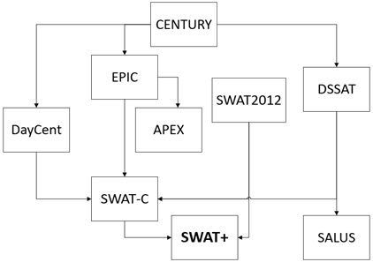
SWAT+ is a restructured version of the Soil & Water Assessment Tool (SWAT), allowing for more flexible spatial interactions and processes within a watershed than the previous model version (Bieger et al. 2017). SWAT+ is a public domain model jointly developed by USDA ARS and Texas A&M at Blackland Research and Extension Center, under an LGPL-2.1 license (Free Software Foundation 1999).

Figure 3 shows a simplified view of the model’s pedigree. SWAT+ inherited the stable SWAT2012 model, and obtained the soil organic carbon code from SWAT-C (Zhang et al. 2013), which in turn originated from code from the CENTURY and EPIC models.

Figure 3: Model pedigree for SWAT+

8.4 Workflow

SWAT+ will estimate soil organic carbon dynamics from 2008 to the latest available year, and assess the trend resulting from management and conservation practices. The FP will send a modeling request containing field-specific data to the SWAT+ model web service (Figure 4), which will process the request by translating the management inputs, adding location-specific weather, soil parameters, and other required data inputs required for SWAT+ to run. The service will run one simulation for each soil type, returning the modeling results that will be processed by the FP to present the final output to users. FP inputs to the SWAT+ model service match reasonably well with inputs to the USDA Water Erosion Prediction Project (WEPP) (Flanagan et al. 2024) and the Wind Erosion Prediction System (WEPS) (Wagner 2013) models, which are used by the FP for the Soil Conservation metric. Some inputs required for the Water Quality metric will also be used for SWAT+ model runs.

Figure 4: High-level modeling workflow for SWAT+

The USDA Conservation Effect Assessment Project (CEAP), authorized in the Farm Bill since 2002, runs SWAT+ to model water quality and other resource effects on 2,000+ HUC-8 watersheds across the country to assess the impact of conservation practices on agriculture and the broader environment (Mausbach and Dedrick 2004; Duriancik et al. 2008). The CEAP work produces soft-calibrated input parameter datasets for crop biomass and water balance specific to each HUC-8. The FP SWAT+ model service will leverage these input parameters to realistically simulate the farmer’s cropping system. As necessary, additional hard calibrations will adjust carbon and nitrogen flux parameters to achieve sample and research study soil organic carbon targets by region and soil strata.

Important

What are soft and hard data for model calibration?

A rich conceptual discussion of soft and hard calibration data for environmental modeling can be found in Seibert and McDonnell (2002). Specific to the SWAT+ ecosystem, soft and hard calibration strategies have been employed by several researchers (Čerkasova et al. 2023; Yen et al. 2016; Chawanda et al. 2020).

Čerkasova et al. (2023) defines the terms as follows:

• Soft data are defined as information on individual processes within a budget [system] that may not be directly measured within the study area.
• Hard data are more rigorous, representing observational data directly comparable with some element in the model.

Arnold et al. (2015) includes examples of soft data, such as average depth of groundwater table, average crop/vegetation leaf area index, annual rates of denitrification from the literature, or county-level crop yields from USDA NASS. Hard calibration data would include measurements of streamflow, groundwater levels, or soil moisture for a given area.

The SWAT+ model service quantifies soil carbon stock to a specified depth in the soil profile, the default set to 30 cm. The model simulates soil carbon stock, fluxes among carbon and nitrogen pools, and CO₂ emissions by soil horizon, as well as carbon and nitrogen loss through runoff, lateral flow, and percolation through the soil profile.

Agroecosystem models such as SWAT+ generally lack sufficient measured SOC time series data coverage (hard data) for comprehensive regional calibration. However, exclusive reliance on hard data can lead to misrepresenting underlying processes as calibration targets are met. Calibrating parameters to underlying process targets (water balance, biomass/yield, nutrient balance, etc.) using soft data (expert knowledge, soil samples, crop survey data, etc.) enables more realistic simulations. SWAT+ model calibration uses a combination of soft and hard data according to the NRCS Land Resource Region (LRR), or to the major land resource area (MLRA) or HUC-8 watershed, depending on data availability. Model validation uses the measured datasets from long-term studies across the country supporting other validation efforts for ecosystem service crediting and delivery.

Prior to calling the SWAT+ model service, FP will use the Cropland Data Layer to fill in a yearly cash crop sequence for a given field boundary, adding typical or user-specified plant, harvest, fertilization, tillage, and other management activities to an input object for the model service. The process of creating the management object assumes that high-quality user-specified inputs override typical pre-filled inputs. Based on the FP request, which provides field location, the SWAT+ model service will resolve valid soil components in the field from the NRCS Soil Data Mart (SDM), adding soil component identifiers in the service request. The FP request may specify a practice change year to separate a baseline period and facilitate a before/after analysis.

Upon receipt of the web service request from the FP, the SWAT+ model service will conduct data quality checks to verify readiness for model simulation. The service will intersect location coordinates with gridMET weather data (Abatzoglou 2013) to create an input file containing daily values for precipitation, temperature, solar radiation, relative humidity, and wind speed from 2008 through the most recent year.

The service will create input files for each soil component specified in the request, including bulk density, water holding capacity, soil texture, pH, organic matter, percolation, and other required parameters. The service will process the management object to files and formats needed for the model. It will update other model input files on the fly, reflecting field conditions. Finally, the service will feed the inputs to the SWAT+ model, running simulations for each valid soil component in the field.

For each simulation, the SWAT+ model will initialize structural and metabolic litter pools, microbial (active), slow (resistant), and passive (mineral adsorbed) soil organic carbon (SOC) pools using the SDM organic matter parameter (or on-site sampled SOC data) and ratios derived from CENTURY model research. The model will stabilize output through a seven-year warm-up simulation period (2008 to 2014). The model will grow each crop specified in the management object, allocating biomass to crop yield, leaving the field, aboveground, and root residue, and then partitioning residue to structural and metabolic litter above and below ground. The model simulates the carbon and nitrogen (C + N) dynamics from the litter pools to the microbial and slow SOC pools, with microbes in the microbial pool fluxing C + N to and among decomposition-resistant slow and very resistant passive SOC pools. Each step respires CO₂ while also losing C + N to solution in runoff, percolation, and lateral flow. SWAT+ quantifies daily litter and SOC for each pool on the soil surface and on all soil profile horizons. Sequestered carbon is considered the sum of microbial, slow, and passive SOC below the soil surface.

Once a simulation is complete, the SWAT+ model web service will post-process the output to a response payload back to FP containing SOC stock results from 2015 onward at specified soil depths and other outputs needed to populate Soil Carbon metric reports. The standard reporting depth will be 30-cm; however, SWAT+ produces output for several depth options. The service will also produce a time-limited simulation archive for technical support and problem diagnosis. Future service enhancements will include options to project SOC trends 10 or more years into the future and compare SOC trends to a baseline.

For FP v5, the Energy Use, GHG Emissions, and Soil Carbon metrics will provide results for the assessment of various management practices intended to reduce energy use and GHG emissions, and increase SOC stocks:

• Reducing the number and intensity of tillage activities.
• Increasing sources of carbon through cover cropping.
• Growing perennial crops (alfalfa).
• Implementing perennial conservation cover.
• Impact of residue management (baling, grazing, setting on fire, etc.).
• Organic matter additions (animal manure, green manure, compost, biosolids).

Although tillage can incorporate large amounts of surface residue into the soil, it exposes sequestered carbon and root litter to increased microbial decomposition. This leads to higher CO₂ emissions, usually to the point of net SOC losses with high disturbance tillage. On the other hand, reduced and no-till management might lead to net gains on some soils and regions. Introducing deep-rooted perennials (e.g., alfalfa) to the cropping sequence adds residue and increases SOC in lower soil layers. Increasing cropping intensity with cover crops puts more live roots in the ground during the year, resulting in higher root residue litter pools and a higher likelihood of increasing SOC.

8.5 Crop growth module

SWAT+ can simulate crop growth for one-at-a-time and simultaneous crops within a given field (Bieger et al. 2017). The module uses schedule files with activities, dates, heat units, and decision tables, which are more flexible than the APEX and EPIC models (Arnold et al. 2018). The crop growth module is flexible enough to allow for intercropping of commodity crops and cover crops. The plant growth database distributed with SWAT+ includes parameters for the most common plant species (row crops, vegetables, trees, and grasses).

SWAT+ uses the date input in the management operation file to simulate the crop growth cycle. It will use a fraction of potential heat units if no date is provided. Scheduling by heat units allows the model to time the operation as a function of temperature. Using heat units will allow the management operation to be used anywhere in the watershed, and depending on the weather in each region or the changing weather from year to year, the model will adjust the timing of the cycle each year.

8.6 Soil organic carbon module

The SWAT+ soil organic carbon module was based on the SWAT-C model (Zhang et al. 2013). SWAT-C was developed based on SWAT2012 version 682. SWAT-C incorporated terrestrial soil organic matter dynamics from the CENTURY and EPIC models and aquatic carbon cycling processes from QUAL2K and CE-QUAL-W2 (Du et al. 2019) into SWAT2012, enabling the assessment of carbon and nitrogen fluxes on cultivated land through water courses and wetlands in a watershed. New algorithms have been added to enable the model to represent the coupled terrestrial and aquatic carbon cycle at the watershed scale. SWAT-C calculated SOC based on the combined factors Izaurralde et al. (2006) modified to represent biochemical and hydroclimatic processes influencing the carbon cycle and balance in an agroecosystem.

In SWAT+, the distribution of C and N across soil layers (Figure 5) is divided into five pools (organic and inorganic) as in CENTURY (with the turnover time included):

• Metabolic litter (<1 year): The readily decomposable organic matter from plants, such as dead organic matter or leaves with high nitrogen content and animal waste.
• Structural litter (1 year): It refers to the more resistant, slowly decomposing organic material, like lignin.
• Microbial biomass (<1 year): The living mass of microorganisms such as bacteria, fungi, protozoa, and nematodes within the soil, responsible for breaking down organic matter like litter into simpler compounds.
• Slow humus (5 years): Slow humus is partially decomposed organic matter that breaks down moderately over several years.
• Passive humus (200+ years): Passive humus is a highly stable, old organic matter that decomposes over centuries.

Figure 5: Carbon pools and fluxes modeled by SWAT+, from Liang et al. (2022)

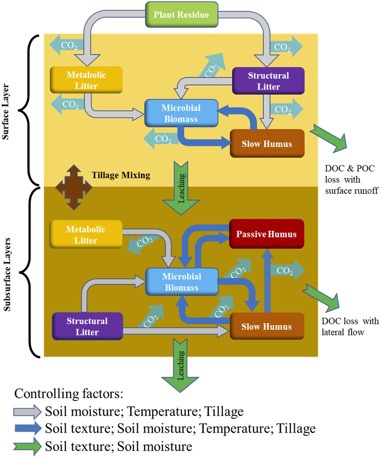
Soil organic carbon turnover rates depend on nonlinear processes influenced by environmental and management factors (Liang et al. 2022). Carbon and nitrogen flow among these pools through various pathways influenced by biotic and abiotic factors (Figure 5). The decomposition and transformation rates of C and N among these pools are affected by soil temperature, soil water content, soil texture, land management practices, soil aeration, and conditions such as the soil C/N ratio. Carbon flow within the soil profile is associated with hydrologic processes such as percolation, lateral flow, and soil erosion. Tillage and percolation can redistribute SOC vertically, while lateral flow and erosion redistribute SOC laterally. Figure 5 illustrates the addition, decomposition, and transformation of SOC among the different pools and its flow in various soil layers represented in SWAT-C.

8.7 Model setup

As explained in Section 8.2, the development team at CSU has added SWAT+ to their Cloud Services Integration Platform (CSIP) (David et al. 2014) to run soil organic carbon simulations. The CSIP service appends climate, soils, and management data for a given field, runs the model at a computational scale, and post-processes results into the Fieldprint Platform. The same version of the SWAT+ model implemented by CSU via CSIP can be found in a GitHub repository (Arnold et al. 2024).

8.7.1 Data inputs

• Data and resources developed by the National Agroecosystem Model (NAM), a comprehensive model that uses SWAT+ to simulate staple crop yields across the contiguous United States (Čerkasova et al. 2023).
• CRLMOD reference data (Kucera and Coreil 2023)
• Soil Survey Geographic Database (NRCS)
• Land use map, digital elevation model, watershed outlets, reservoirs, and soil map to delineate watersheds and define Hydrological Response Units (HRUs) and Landscape Units.
• Climate data such as daily precipitation, minimum and maximum temperature, solar radiation, relative humidity, and wind speed (Abatzoglou 2013).
• Cropland Data Layer for detection of cash crops and land use (Boryan et al. 2011).
• Crop management data from growers Section 5.6.

Figure 6 shows the management files that can go into SWAT+. The implementation of the FP will use select modules.

Figure 6: Land cover and management files in SWAT+, from Bieger et al. (2017)

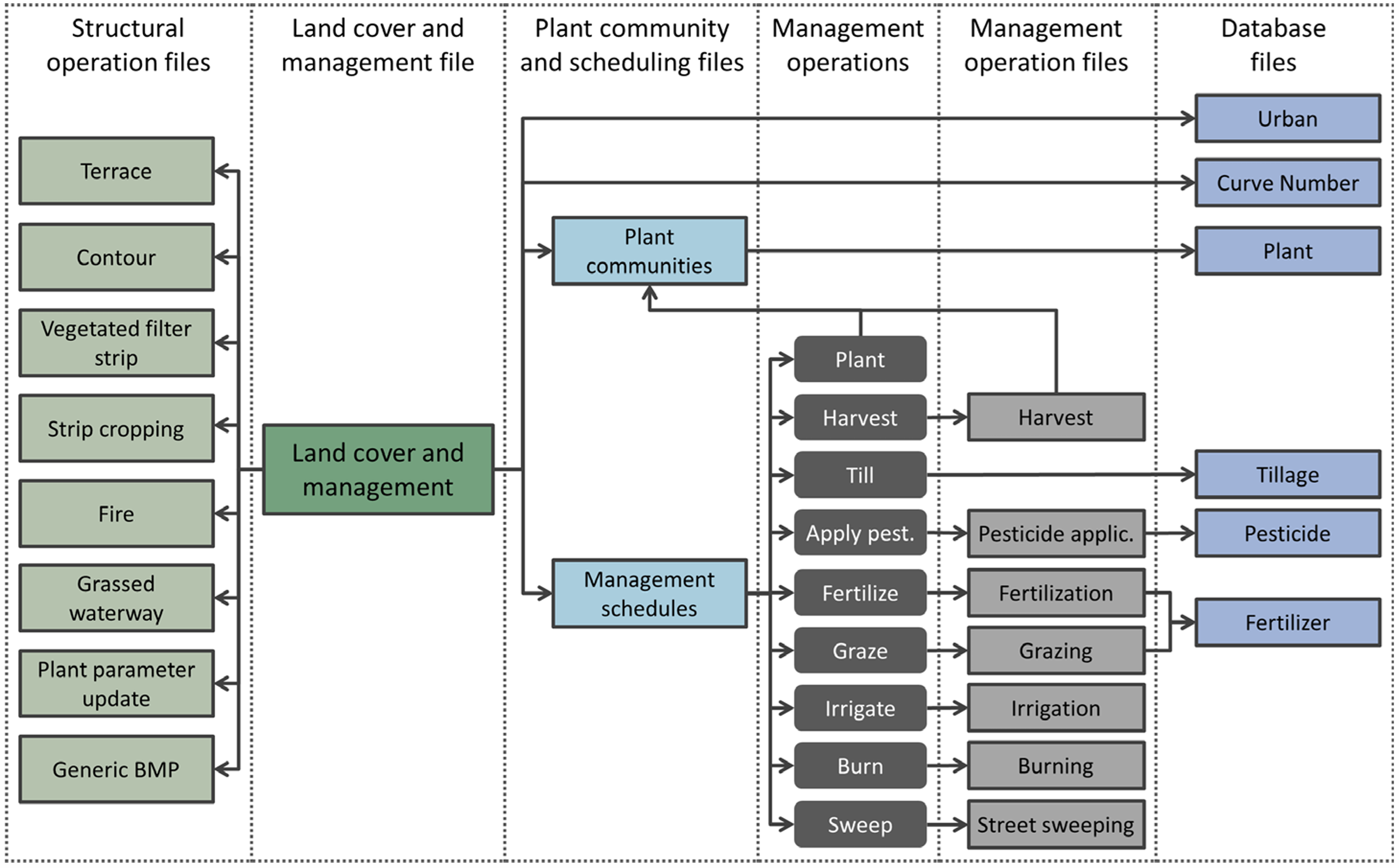
8.8 Definition

With the implementation of SWAT+, annual sequestered soil organic carbon stock changes can be expressed either as elemental carbon or carbon dioxide equivalents as follows:

\[ \Delta SOC = \Delta SOC_{microbial} + \Delta SOC_{slow} + \Delta SOC_{passive} \] Where:

• \(\Delta SOC\) = Soil organic carbon (SOC) stock changes from consecutive years.
• \(\Delta SOC_{microbial}\) = SOC stock changes from the mass of microorganisms within the soil.
• \(\Delta SOC_{slow}\) = SOC stock changes from partially decomposed organic matter that breaks down over several years.
• \(\Delta SOC_{passive}\) = SOC stock changes from passive humus that decomposes over centuries.

8.9 Modeling approach

The modeling approach from Colorado State University for SWAT+ follows the principles from Del Grosso et al. (2011) to test and review model performance:

1. Conduct an initial model run using best estimates of weather, soil, and plant parameters.
2. Are plant growth, soil carbon, and grain yields reasonable?
   • If not, refer back to initial input parameters to ensure they are correct (e.g., maximum and minimum temperatures, precipitation, crop type, soil profile characteristics).
3. Are soil water content and soil N correct?
   • If not, adjust soil hydraulic properties (e.g., Ksat, percent sand, percent clay, and bulk density.
4. Are ET [evapotranspiration], leaching rates, and runoff correct?
   • If not, adjust any number of water conductance parameters. These include but are not limited to Ksat, permanent wilting point, and field capacity, rooting depth, infiltration rates, stomatal conductance, etc.
5. Are fertilizer applications and cultivation methods correct?
   • The model is very sensitive to fertilizer additions. Slight variations can cause major differences in plant production, so ensure appropriate conversions have been made, if necessary.
6. Are site parameters accurate?
   • If not, refer to site input file and validate climate, soils, and water information.
7. Are trace gas emissions reasonable?
   • If not, refer to the amount of N availability in soil, plant N demand, and soil water information.
8. Are plant growth, soil carbon, and grain estimates still correct?
   • If not, recalibrate parameters related to plant production and soil processes.

8.10 Future SWAT+ developments

• The SWAT-C N₂O component could be integrated into SWAT+, enabling the FP to use a Tier 3 approach to estimate N₂O emissions as part of the GHG Emissions metric.
• Researchers are actively working on the development of a SWAT+ module to simulate CH₄ emissions from flooded rice production. Eventually, this module could replace the Tier 2 method for CH₄ emission estimations from rice production.
• SWAT+ could support the Water Quality metric by providing quantitative estimates of nitrogen and phosphorus losses.

8.11 Uncertainty quantification

SWAT+ developers will apply computational frameworks to analyze the uncertainty in model estimates of soil carbon stocks, with the goal of developing uncertainty bounds around field-level estimates. The uncertainty sources in models such as SWAT+ are several, including model parameters, input data, model structure, and measurement data used for training and testing the model (Tasdighi et al. 2018).

Developers will use documented approaches applied to SWAT2012, the previous model version before SWAT+, to produce uncertainty bounds (Tasdighi et al. 2018; Arabi, Govindaraju, and Hantush 2007; Tasdighi, Arabi, and Harmel 2018; Arnold et al. 2012).

8.12 General considerations of agroecosystem models

Del Grosso et al. (2011) provide a useful summary of considerations:

• No perfect method exists to measure variables of interest in agroecosystems.
• There are limitations when ground-based measurements at small spatial and temporal scales are used to infer variables at larger scales.
• Models can provide complete spatial and temporal coverage; however, models are a simplification of reality.
• There is uncertainty in both the inputs used to run models and the measurements to test model outputs.
• Some model inputs have less uncertainty than others (e.g., grain yield vs gas fluxes).
• Model results are nearly always mixed; some outputs compare well against measurements in some conditions, but not all.

9 Impact on user burden for data collection

The transition from FP v4.2 to v5 represents a significant enhancement on many fronts. FP v5 will enable users to provide the same level of detail from FP v4.2 in a more explicit manner. The module to create crop rotation templates in FP v4.2 will be retired, and the FP v5 engine will create the crop rotation templates based on the user responses.

With FP v5, many user inputs can be derived through the reorganized user interface in ways that we could not do with FP v4.2. New user inputs are related to the following sources:

• Cover cropping activities.
• Manure applications.
• Soil N₂O.

We will be able to repurpose or rewrite several FP v4.2 inputs, keeping the net increase of questions to a reasonable number.

10 Known limitations and potential enhancements

• Except for cotton, there is currently no accounting for co-products or by-products. This could be developed with stakeholder collaborations.
• There is currently no accounting method for on-farm energy generation (e.g., solar or wind power). This could be developed with stakeholder collaborations. Solar and wind power generation would account for the manufacturing process and energy storage system, including the impact of fluorinated gases, steel, and other primary components.
• Impact factors are meant to represent average properties of inputs and activities. We currently do not host impact factors from branded data, such as the impact factors of a given fertilizer product marketed by a corporation. Field to Market is willing to collaborate with scientists and organizations to better represent their cropping systems, equipment used, and inputs applied. The Metrics Committee plans to provide guidance about incorporating branded impact factors into the Fieldprint Platform.
• The Fieldprint Platform cannot model the impact of agricultural inputs if they are not part of widely recognized publications, such as the GHG quantification methods from Ogle et al. (2024) or IPCC (2019). For example, it is not currently possible to quantify the enhanced soil carbon sequestration of some products claiming to do so. Similarly, for soil N₂O emissions, the methods account for the impact of N inhibitors and slow-release N fertilizers, which are modeled with methods from Ogle et al. (2024), but no N₂O reductions can be modeled with products that are not N inhibitors or slow-release N fertilizers. Field to Market does not conduct field testing of agricultural inputs.
• The Fieldprint Platform does not currently model the impact of biochar applications. This could be developed with stakeholder collaborations.
• The Fieldprint Platform currently lacks a method to account for energy use and associated GHG emissions for corn silage and alfalfa hay post-harvest processing, such as bagging, making square or round modules, etc. This could be developed with stakeholder collaborations.
• We are currently assessing how to use soil organic carbon samples to initialize SWAT+. We plan to release recommendations at a later date.
• The method for CH₄ emissions from flooded rice cultivation does not have explicit guidance to account for rice ratooning emissions. We propose a solution in Supplementary Material.
• The direct land use change method does not currently consider the conversion from wetland to cropland. We plan to add this to a future release if there are requests from Fieldprint Platform users or if we start encountering CDL detection of wetlands during regular Fieldprint Platform usage.
• Transportation of agricultural inputs represents a minimal source of energy use and GHG emissions; this source includes the transportation distance from the processing gate to the retailer, and it is attributed to the upstream system boundary. FP v5 will include a fixed factor of 196 km or 122 miles for transportation of ag inputs (BLS 2017) without the need for user input.

References

Abatzoglou, John T. 2013. “Development of Gridded Surface Meteorological Data for Ecological Applications and Modelling.” International Journal of Climatology 33 (1): 121–31.

ANL. 2024. “Greenhouse Gases, Regulated Emissions, and Energy Use in Technologies Model (GREET).” Argonne National Laboratory. https://www.energy.gov/eere/rd-greet-life-cycle-assessment-model.

Arabi, Mazdak, Rao S Govindaraju, and Mohamed M Hantush. 2007. “A Probabilistic Approach for Analysis of Uncertainty in the Evaluation of Watershed Management Practices.” Journal of Hydrology 333 (2-4): 459–71.

Arena, Marika, Giovanni Azzone, and Antonio Conte. 2013. “A Streamlined LCA Framework to Support Early Decision Making in Vehicle Development.” Journal of Cleaner Production 41: 105–13.

Arinze, EA, S Sokhansanj, GJ Schoenau, and FG Trauttmansdorff. 1996. “Experimental Evaluation, Simulation and Optimization of a Commercial Heated-Air Batch Hay Drier: Part 1, Drier Functional Performance, Product Quality, and Economic Analysis of Drying.” Journal of Agricultural Engineering Research 63 (4): 301–14.

Arnold, Jeffrey G, Katrin Bieger, Michael J White, Raghavan Srinivasan, John A Dunbar, and Peter M Allen. 2018. “Use of Decision Tables to Simulate Management in SWAT+.” Water 10 (6): 713.

Arnold, Jeffrey G, Natalja Čerkasova, Michael J White, Ryan Bailey, Kelly Thorp, Jaehak Jeong, Xuesong Zhang, et al. 2024. “Soil and Water Assessment Tool Plus (SWAT+).” https://github.com/swat-model/swatplus.

Arnold, Jeffrey G, Daniel N Moriasi, Philip W Gassman, Karim C Abbaspour, Michael J White, Raghavan Srinivasan, Chinnasamy Santhi, et al. 2012. “SWAT: Model Use, Calibration, and Validation.” Transactions of the ASABE 55 (4): 1491–1508.

Arnold, Jeffrey G, Mohamed A Youssef, Haw Yen, Michael J White, Aleksey Y Sheshukov, Ali M Sadeghi, Daniel N Moriasi, et al. 2015. “Hydrological Processes and Model Representation: Impact of Soft Data on Calibration.” Transactions of the ASABE 58 (6): 1637–60.

Audsley, Eric, K Stacey, DJ Parsons, and AG Williams. 2009. “Estimation of the Greenhouse Gas Emissions from Agricultural Pesticide Manufacture and Use.” https://doi.org/10.13140/RG.2.1.5095.3122.

Baldocchi, Dennis, Eva Falge, Lianhong Gu, Richard Olson, David Hollinger, Steve Running, Peter Anthoni, et al. 2001. “FLUXNET: A New Tool to Study the Temporal and Spatial Variability of Ecosystem-Scale Carbon Dioxide, Water Vapor, and Energy Flux Densities.” Bulletin of the American Meteorological Society 82 (11): 2415–34.

Bandekar, Prathamesh A, Ben Putman, Greg Thoma, and Marty Matlock. 2022. “Cradle-to-Grave Life Cycle Assessment of Production and Consumption of Pulses in the United States.” Journal of Environmental Management 302: 114062.

Barber, Andrew. 2004. “Seven Case Study Farms: Total Energy & Carbon Indicators for New Zealand Arable & Outdoor Vegetable Production.” AgriLINK New Zealand Ltd 288.

Bastviken, David, Julie Wilk, Nguyen Thanh Duc, Magnus Gålfalk, Martin Karlson, Tina-Simone Neset, Tomasz Opach, Alex Enrich-Prast, and Ingrid Sundgren. 2022. “Critical Method Needs in Measuring Greenhouse Gas Fluxes.” Environmental Research Letters 17 (10): 104009.

Bieger, Katrin, Jeffrey G Arnold, Hendrik Rathjens, Michael J White, David D Bosch, Peter M Allen, Martin Volk, and Raghavan Srinivasan. 2017. “Introduction to SWAT+, a Completely Restructured Version of the Soil and Water Assessment Tool.” JAWRA Journal of the American Water Resources Association 53 (1): 115–30.

Blankenship, Paul D, and Victor Chew. 1979. “Peanut Drying Energy Consumption.” Peanut Science 6 (1): 10–13.

BLS. 2017. “Commodity Flow Survey (CFS).” Bureau of Transportation Statistics. https://www.bts.gov/cfs.

Bormann, Nancy Bohl, Erin Cortus, Melissa Wilson, Kevin Silverstein, Larry Gunderson, and Kevin Janni. 2024. “ManureDB-National Database of Manure Nutrient Content and Other Characteristics: 1998-2023.”

Boryan, Claire, Zhengwei Yang, Rick Mueller, and Mike Craig. 2011. “Monitoring US Agriculture: The US Department of Agriculture, National Agricultural Statistics Service, Cropland Data Layer Program.” Geocarto International 26 (5): 341–58.

BTS. 2024. “Combination Truck Fuel Consumption and Travel.” Bureau of Transportation Statistics. https://www.bts.gov/content/combination-truck-fuel-consumption-and-travel.

Carlson, Jack R. 2016. “The Soil Conditioning Index Model Service.” https://docs.lib.purdue.edu/cgi/viewcontent.cgi?referer=&httpsredir=1&article=1111&context=agroenviron.

Čerkasova, Natalja, Michael White, Jeffrey Arnold, Katrin Bieger, Peter Allen, Jungang Gao, Marilyn Gambone, Manyowa Meki, James Kiniry, and Philip W Gassman. 2023. “Field Scale SWAT+ Modeling of Corn and Soybean Yields for the Contiguous United States: National Agroecosystem Model Development.” Agricultural Systems 210: 103695.

Chawanda, Celray James, Jeffrey Arnold, Wim Thiery, and Ann van Griensven. 2020. “Mass Balance Calibration and Reservoir Representations for Large-Scale Hydrological Impact Studies Using SWAT+.” Climatic Change 163: 1307–27.

Czyrnek-Delêtre, Magdalena M., Beatrice M. Smyth, and Jerry D. Murphy. 2017. “Beyond Carbon and Energy: The Challenge in Setting Guidelines for Life Cycle Assessment of Biofuel Systems.” Renewable Energy 105: 436–48. https://doi.org/https://doi.org/10.1016/j.renene.2016.11.043.

David, Olaf, Jeffrey Arnold, Natalja Čerkasova, Eric Coronel, Jack Carlson, Frank Geter, and Xuesong Zhang. 2024. “SWAT+ Carbon.” 2024 SWAT Conference (Strasbourg, France). https://swat.tamu.edu/media/0t5c4bul/olaf.pdf.

David, Olaf, Wes Lloyd, Ken Rojas, Mazdak Arabi, Frank Geter, James C Ascough II, Tim Green, George Leavesley, and Jack Carlson. 2014. “Model-as-a-Service (MaaS) Using the Cloud Services Innovation Platform (CSIP).”

Del Grosso, Stephen J, WJ Parton, CA Keough, and M Reyes-Fox. 2011. “Special Features of the DayCent Modeling Package and Additional Procedures for Parameterization, Calibration, Validation, and Applications.” Methods of Introducing System Models into Agricultural Research 2: 155–76.

Du, Xinzhong, Xuesong Zhang, Rajith Mukundan, Linh Hoang, and Emmet M Owens. 2019. “Integrating Terrestrial and Aquatic Processes Toward Watershed Scale Modeling of Dissolved Organic Carbon Fluxes.” Environmental Pollution 249: 125–35.

Duriancik, Lisa F, Dale Bucks, James P Dobrowolski, Tom Drewes, S Diane Eckles, Leonard Jolley, Robert L Kellogg, et al. 2008. “The First Five Years of the Conservation Effects Assessment Project.” Journal of Soil and Water Conservation 63 (6): 185A–197A.

EC–European Commission. 2010. “2010/335/: Commission Decision of 10 June 2010 on Guidelines for the Calculation of Land Carbon Stocks for the Purpose of Annex v to Directive 2009/28/EC (Notified Under Document c(2010) 3751).” Official Journal of the European Union. https://eur-lex.europa.eu/eli/dec/2010/335/oj.

Eisenhauer, Dean E, Derrel L Martin, Derek M Heeren, and Glenn J Hoffman. 2021. Irrigation Systems Management. American Society of Agricultural; Biological Engineers (ASABE).

European Chemicals Agency. 2024. “Search for Chemicals.” https://echa.europa.eu/information-on-chemicals.

Fava, Jim, Steven Baer, and Joyce Cooper. 2011. “Green (Er) Product Standard Trends in North America.” Journal of Industrial Ecology 15 (1): 9–12.

Fertilizers Europe. 2024. “Carbon Footprinting in Fertilizer Production.” https://www.fertilizerseurope.com/initiatives/carbon-footprint-calculator/.

Field to Market. 2021. Press Releases. https://fieldtomarket.org/field-to-market-launches-fieldprint-platform-4-0-with-enhanced-science-to-assess-nutrient-loss-pathways-and-estimate-soil-carbon-sequestration/.

Flanagan, Dennis C, James R Frankenberger, Chris S Renschler, Chris B Coreil, Olaf David, Anurag Srivastava, Sadia A Jame, Ryan P McGehee, et al. 2024. “Water Erosion Prediction Project (WEPP) Model 2024 Status.” In 2024 ASABE Annual International Meeting, 1. American Society of Agricultural; Biological Engineers.

Free Software Foundation. 1999. “GNU Lesser General Public License V2.1.” https://www.gnu.org/licenses/old-licenses/lgpl-2.1-standalone.html.

Gaidajis, Georgios, and Ilias Kakanis. 2020. “Life Cycle Assessment of Nitrate and Compound Fertilizers Production—a Case Study.” Sustainability 13 (1): 148.

Green, MR. 1987. “Energy in Pesticide Manufacture, Distribution and Use.” Energy in Plant Nutrition and Pest Control.

Guan, Kaiyu, Zhenong Jin, Bin Peng, Jinyun Tang, Evan H DeLucia, Paul C West, Chongya Jiang, et al. 2023. “A Scalable Framework for Quantifying Field-Level Agricultural Carbon Outcomes.” Earth-Science Reviews 243: 104462.

Hanson, Wes L, Cortney Itle, Kara Edquist, et al. 2024. “Quantifying Greenhouse Gas Fluxes in Agriculture and Forestry: Methods for Entity-Scale Inventory.”

Heidari, Mohammad Davoud, Damien Mathis, Pierre Blanchet, and Ben Amor. 2019. “Streamlined Life Cycle Assessment of an Innovative Bio-Based Material in Construction: A Case Study of a Phase Change Material Panel.” Forests 10 (2): 160.

Hoffman, Glenn J, Terry A Howell, and Kenneth H Solomon. 1990. Management of Farm Irrigation Systems.

Hunt, Robert G, Terrie K Boguski, Keith Weitz, and Aarti Sharma. 1998. “Case Studies Examining LCA Streamlining Techniques.” The International Journal of Life Cycle Assessment 3: 36–42.

IPCC. 2019. “2019 Refinement to the 2006 IPCC Guidelines for National Greenhouse Gas Inventories.” Agriculture, Forestry and Other Land Use. IPCC Geneva, Switzerland:

IPCC. 2022. “IPCC Emission Factor Database.” https://www.ipcc-nggip.iges.or.jp/EFDB/main.php.

———. 2023. “Climate Change 2023: Synthesis Report. Contribution of Working Groups i, II and III to the Sixth Assessment Report of the Intergovernmental Panel on Climate Change.” Core Writing Team, Lee, H. And Romero, J. (Eds.). https://doi.org/10.59327/IPCC/AR6-9789291691647.

ISO. 2006. “Environmental management — Life cycle assessment — Principles and framework.” ISO 14040:2006. International Organization for Standardization.

Izaurralde, RC, Jimmy R Williams, William B McGill, Norman J Rosenberg, and MC Quiroga Jakas. 2006. “Simulating Soil c Dynamics with EPIC: Model Description and Testing Against Long-Term Data.” Ecological Modelling 192 (3-4): 362–84.

Kehoe, Laura, Alfredo Romero-Muñoz, Ester Polaina, Lyndon Estes, Holger Kreft, and Tobias Kuemmerle. 2017. “Biodiversity at Risk Under Future Cropland Expansion and Intensification.” Nature Ecology & Evolution 1 (8): 1129–35.

Kløverpris, Jesper Hedal, Claus Nordstrøm Scheel, Jannick Schmidt, Brian Grant, Ward Smith, and Murray J Bentham. 2020. “Assessing Life Cycle Impacts from Changes in Agricultural Practices of Crop Production: Methodological Description and Case Study of Microbial Phosphate Inoculant.” The International Journal of Life Cycle Assessment 25: 1991–2007.

Kucera, Michael J., and Christopher B. Coreil. 2023. “Overview of USDA-NRCS Erosion Prediction Technology and Conservation Resources - Land Management Operations Database and Use.” Soil Erosion Research Under a Changing Climate, January 8-13, 2023, Aguadilla, Puerto Rico, USA. https://doi.org/10.13031/soil.23007.

LEIF. 2025. “Impact Factors.” https://www.leifllc.com/.

Liang, Kang, Junyu Qi, Xuesong Zhang, and Jia Deng. 2022. “Replicating Measured Site-Scale Soil Organic Carbon Dynamics in the US Corn Belt Using the SWAT-c Model.” Environmental Modelling & Software 158: 105553.

Liu, Xinyu, Hao Cai, Hoyoung Kwon, and Michael Wang. 2023. “Feedstock Carbon Intensity Calculator (Fd-Cic): Users’ Manual and Technical Documentation.” Argonne National Laboratory (ANL), Argonne, IL (United States).

Mausbach, Maurice J, and Allen R Dedrick. 2004. “The Length We Go: Measuring Environmental Benefits of Conservation Practices.” Journal of Soil and Water Conservation 59 (5): 96A–.

Mendoza Beltran, Angelica, Claus Nordstrøm Scheel, Nuala Fitton, Jannick Schmidt, and Jesper Hedal Kløverpris. 2021. “Assessing Life Cycle Environmental Impacts of Inoculating Soybeans in Argentina with Bradyrhizobium Japonicum.” The International Journal of Life Cycle Assessment 26: 1570–85.

National Renewable Energy Laboratory. 2012. “U.s. Life Cycle Inventory Database.”

Newell, David B, Eite Tiesinga, et al. 2019. “The International System of Units (SI).” NIST Special Publication 330: 1–138.

NRCS. “Soil Survey Staff.” United States Department of Agriculture. https://websoilsurvey.nrcs.usda.gov/.

Ogle, Stephen M, Paul R Adler, Gary Bentrup, Justin Derner, Grant Domke, Stephen Del Grosso, Johannes Lehmann, Michele Reba, and Dominic Woolf. 2024. “Chapter 3: Quantifying Greenhouse Gas Sources and Sinks in Cropland and Grazing Land Systems.” In: Hanson, Wes L.; Itle, Cortney; Edquist, Kara, Eds. Quantifying Greenhouse Gas Fluxes in Agriculture and Forestry: Methods for Entity-Scale Inventory. Technical Bulletin Number 1939, 2nd Edition. Washington, DC: US Department of Agriculture, Office of the Chief Economist. 6-1-6-23. Chapter 3. 1939: 3–1.

Panigrahi, Shubham Subrot, Kaushik Luthra, Chandra B Singh, Griffith Atungulu, and Kenny Corscadden. 2023. “On-Farm Grain Drying System Sustainability: Current Energy and Carbon Footprint Assessment with Potential Reform Measures.” Sustainable Energy Technologies and Assessments 60: 103430.

Parker, BF, GM White, MR Lindley, RS Gates, M Collins, S Lowry, and TC Bridges. 1992. “Forced-Air Drying of Baled Alfalfa Hay.” Transactions of the ASAE 35 (2): 607–15.

Pelton, Rylie. 2018. “Spatial Greenhouse Gas Emissions from US County Corn Production.” The International Journal of Life Cycle Assessment 24 (1): 12–25. https://doi.org/10.1007/s11367-018-1506-0.

Pier, F, S Trude, A Kyle, C William, D Jean-Louis, F David, DJ Lunt, et al. 2021. “Chapter 7: The Earth’s Energy Budget, Climate Feedbacks and Climate Sensitivity.” Climate Change, 132.

Pimentel, David. 2019. Handbook of Energy Utilization in Agriculture. CRC press.

Richards, Meryl B. 2018. “Measure the Chain: Tools for Assessing GHG Emissions in Agricultural Supply Chains.” https://www.ceres.org/resources/reports/measure-chain-tools-managing-ghg-emissions-agricultural-supply-chains.

Rosa, Lorenzo, Davide Danilo Chiarelli, Maria Cristina Rulli, Jampel Dell’Angelo, and Paolo D’Odorico. 2020. “Global Agricultural Economic Water Scarcity.” Science Advances 6 (18). https://doi.org/10.1126/sciadv.aaz6031.

Sándor, Renáta, Fiona Ehrhardt, Lorenzo Brilli, Marco Carozzi, Sylvie Recous, Pete Smith, Val Snow, et al. 2018. “The Use of Biogeochemical Models to Evaluate Mitigation of Greenhouse Gas Emissions from Managed Grasslands.” Science of the Total Environment 642: 292–306.

Savoie, P, and H Joannis. 2006. “Bidirectional Drying of Baled Hay with Air Recirculation and Cooling.” Canadian Biosystems Engineering 48: 3.

Seibert, Jan, and Jeffrey J McDonnell. 2002. “On the Dialog Between Experimentalist and Modeler in Catchment Hydrology: Use of Soft Data for Multicriteria Model Calibration.” Water Resources Research 38 (11): 23–21.

Shortle, J. S., D. G. Abler, and M. Ribaudo. 2001. “Agriculture and Water Quality: The Issues.” In, 1–18. CABI Publishing. https://doi.org/10.1079/9780851993997.0001.

Sieverding, Heidi, Ermias Kebreab, Jane M. F. Johnson, Hui Xu, Michael Wang, Stephen J. Del Grosso, Stephanie Bruggeman, et al. 2020. “A Life Cycle Analysis (LCA) Primer for the Agricultural Community.” Agronomy Journal 112 (5): 3788–3807. https://doi.org/10.1002/agj2.20279.

Swan, Amy, Mark Easter, Kevin Brown, Mark Layer, and Keith Paustian. 2018. “COMET-Planner: Carbon and Greenhouse Gas Evaluation for USDA-NRCS Conservation Practice Planning.”

Tasdighi, Ali, Mazdak Arabi, and Daren Harmel. 2018. “A Probabilistic Appraisal of Rainfall-Runoff Modeling Approaches Within SWAT in Mixed Land Use Watersheds.” Journal of Hydrology 564: 476–89.

Tasdighi, Ali, Mazdak Arabi, Daren Harmel, and Daniel Line. 2018. “A Bayesian Total Uncertainty Analysis Framework for Assessment of Management Practices Using Watershed Models.” Environmental Modelling & Software 108: 240–52.

Thaler, Evan A., Isaac J. Larsen, and Qian Yu. 2021. “The Extent of Soil Loss Across the US Corn Belt.” Proceedings of the National Academy of Sciences 118 (8). https://doi.org/10.1073/pnas.1922375118.

Tilman, David, and Michael Clark. 2015. “Food, Agriculture & the Environment: Can We Feed the World & Save the Earth?” Daedalus 144 (4): 8–23.

Tools, Hydrogen. 2024. “Hydrogen Analysis Resource Center (HYARC) Calculators.” https://h2tools.org/hyarc/calculator-tools/lower-and-higher-heating-values-fuels.

USDA. 2003. “The Soil Conditioning Index.” Agronomy Technical Note No. 1 (Revised). https://efotg.sc.egov.usda.gov/references/public/WA/A.1Soil_Conditioning_Index.pdf.

———. 2019. “Fertilizer Use and Price.” US Department of Agriculture, Economic Research Service.

USDA NASS. 2024a. “2022 Census of Agriculture Highlights: Farms and Farmland.” https://www.nass.usda.gov/Publications/Highlights/2024/Census22_HL_FarmsFarmland.pdf.

———. 2024b. “Surveys: Agricultural Chemical Use Program.”

USEPA. 2023a. “GHG Emission Factors Hub.” U.S. Environmental Protection Agency. https://www.epa.gov/climateleadership/ghg-emission-factors-hub.

———. 2023b. “Inventory of u.s. Greenhouse Gas Emissions and Sinks: 1990-2021” EPA 430-R-23-002. https://www.epa.gov/ghgemissions/inventory-us-greenhouse-gas-emissions-and-sinks-1990-2021.

———. 2024a. “Emissions & Generation Resource Integrated Database (eGRID).” United States Environmental Protection Agency (EPA).

USEPA. 2024b. “Pesticide Product and Label System Database.” https://ordspub.epa.gov/ords/pesticides/f?p=PPLS:1.

———. 2025. “What Is Grid Gross Loss?” https://www.epa.gov/egrid/frequent-questions-about-egrid#What%20is%20Grid%20Gross%20Loss.

Verghese, Karli L, Ralph Horne, and Andrew Carre. 2010. “PIQET: The Design and Development of an Online ‘Streamlined’LCA Tool for Sustainable Packaging Design Decision Support.” The International Journal of Life Cycle Assessment 15: 608–20.

Wagner, Larry E. 2013. “A History of Wind Erosion Prediction Models in the United States Department of Agriculture: The Wind Erosion Prediction System (WEPS).” Aeolian Research 10: 9–24.

Wang, Michael, Amgad Elgowainy, Uisung Lee, Kwang Hoon Baek, Sweta Balchandani, Pahola Thathiana Benavides, Andrew Burnham, et al. 2023. “Summary of Expansions and Updates in r&d GREET 2023.” Argonne National Laboratory (ANL), Argonne, IL (United States).

Wang, Yixuan, James W Levis, and Morton A Barlaz. 2021. “Development of Streamlined Life-Cycle Assessment for the Solid Waste Management System.” Environmental Science & Technology 55 (8): 5475–84.

Wendt, JW, and S Hauser. 2013. “An Equivalent Soil Mass Procedure for Monitoring Soil Organic Carbon in Multiple Soil Layers.” European Journal of Soil Science 64 (1): 58–65.

Wilson, Melissa L, Scott Cortus, Rachel Brimmer, Jerry Floren, Larry Gunderson, Kristin Hicks, Tim Hoerner, et al. 2022. Recommended Methods of Manure Analysis. University of Minnesota Libraries Publishing.

Yen, Haw, Michael J White, Jeffrey G Arnold, S Conor Keitzer, Mari-Vaughn V Johnson, Jay D Atwood, Prasad Daggupati, et al. 2016. “Western Lake Erie Basin: Soft-Data-Constrained, NHDPlus Resolution Watershed Modeling and Exploration of Applicable Conservation Scenarios.” Science of the Total Environment 569: 1265–81.

Zhang, Xuesong, R. César Izaurralde, Jeffrey G. Arnold, Jimmy R. Williams, and Raghavan Srinivasan. 2013. “Modifying the Soil and Water Assessment Tool to Simulate Cropland Carbon Flux: Model Development and Initial Evaluation.” Science of The Total Environment 463-464 (October): 810–22. https://doi.org/10.1016/j.scitotenv.2013.06.056.