# to install, run
pak::pkg_install("Field-to-Market/fieldprintr")Exploratory Analysis with R
Having results in hand allows analysts to check for mistakes, screen fields for outliers, calculate new information, and prepare reports like this one.
The CD 💿
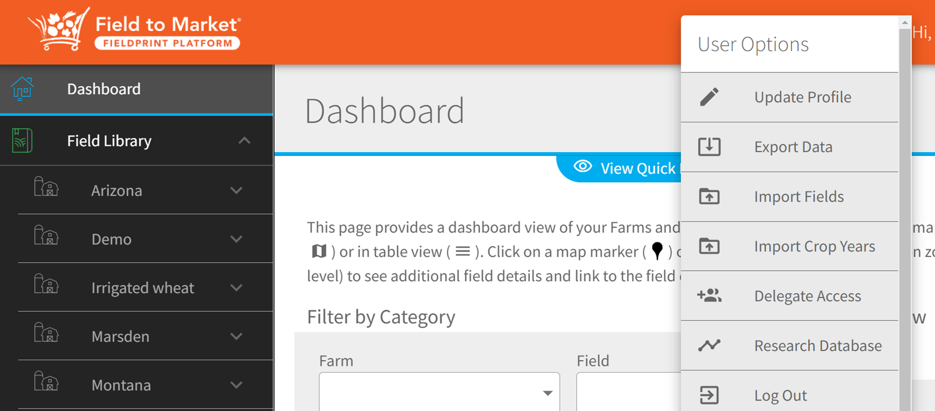
The Comprehensive Data Output File1 is available through the ‘Export Data’ option. The CD is downloaded as an Excel XLSX file.
1 Referred to as “CD” in this training
The Excel workbook contains two worksheets:
Comprehensive Data
-   This sheet contains metadata about the project file, such as

    -   Project name

    -   Date generated

    -   Crops and crop years included
Report DataRow = one grower, one field, one crop, one year
Number of columns varies according to the number of fertilizers and pesticide trips, and with the number of harvest operations for crops like alfalfa.
⬇️Data Dictionary and Column Groupings helper files
Quality assurance
After obtaining your CD output file, consider the following:
is it free of errors?
does it contain potential outliers?
This interactive website2 for quality assurance was built by Eric Coronel to work with CD files. Try it on the example linked above.
2 Again, we trust you to not distribute too widely.
Prep for analysis
fieldprintr
Still very early in development, the fieldprintr R package includes a dummy CD data frame called candyland and a wrapper function for importing CD *.xlsx files into R.

Importing the “CD” file
# load libraries ----------------------------------------------------------
library(fieldprintr)
library(tidyverse)
library(skimr)
#library(scales)

theme_set(theme_bw())

orange <- "#f15d22"
blue <- "#3f8d95"
gray <- "#F1F1F1"

# read in comprehensive data file =============================================
# alternatively, use the readxl::read_xlsx() and janitor::clean_names() functions
raw_data <- fieldprintr::read_ftm_cd(
  "materials/12-09-2022-1234_Comprehensive_Data_Candyland_Farms.xlsx")

# alternatively, use the built-in dataset
candyland
# A tibble: 300 × 422
grower_id field_name field_size_ac farm_serial_number tract_number
<chr> <chr> <dbl> <dbl> <dbl>
1 432 10 22.8 NA 14634
2 441 5a & 5b 59.9 NA 12254
3 427 Bubblegum 1 & 2 41.6 NA 5582
4 427 Bubblegum 11 43.4 NA 16327
5 427 Bubblegum 13 20.7 NA 16327
6 427 Bubblegum 17N 14.5 NA 16327
7 427 Bubblegum 17S 11.6 NA 16327
8 427 Bubblegum 19E 19.5 NA 16327
9 427 Bubblegum 19W 41.1 NA 16327
10 427 Bubblegum 23 23.1 NA 16327
# ℹ 290 more rows
# ℹ 417 more variables: field_number <chr>, location <chr>, state <chr>,
# field_geo_json <chr>, crop_year <chr>, crop <chr>, last_modified_on <dttm>,
# metric_version <chr>, adjusted_yield <dbl>, adjusted_yield_units <chr>,
# land_use_score_acre_yield_units <dbl>, total_soil_loss_year <dbl>,
# soil_conservation_score_ton_acre_year <dbl>,
# water_erosion_ton_acre_year <dbl>, wind_erosion_ton_acre_year <dbl>, …First look at metric scores
Removed 18 irrigated fields to be analyzed separately.
# helper table for column filters
cols_scores <- read_csv("materials/CD-column-groupings.csv") |>
  # filter to just the fieldprint scores
  filter(group == "fieldprint_scores") |>
  pull(variable_clean)


c_metrics <-
  candyland |>
  filter(is_irrigated == "No") |>
  select(crop, crop_year,
         yield = adjusted_yield,
         all_of(cols_scores),
         # remove the character columns
         -energy_use_score_units, -ghg_score_units,
         # remove metrics that are not used (ex irrigation)
         -contains("irrigation"))

# Summary statistics
skimr::skim(c_metrics)| Name | c_metrics |
| Number of rows | 282 |
| Number of columns | 10 |
| _______________________ | |
| Column type frequency: | |
| character | 2 |
| numeric | 8 |
| ________________________ | |
| Group variables | None |
Data summary
Variable type: character
| skim_variable | n_missing | complete_rate | min | max | empty | n_unique | whitespace |
|---|---|---|---|---|---|---|---|
| crop | 0 | 1 | 7 | 13 | 0 | 4 | 0 |
| crop_year | 0 | 1 | 4 | 4 | 0 | 3 | 0 |
Variable type: numeric
| skim_variable | n_missing | complete_rate | mean | sd | p0 | p25 | p50 | p75 | p100 | hist |
|---|---|---|---|---|---|---|---|---|---|---|
| yield | 0 | 1 | 54.06 | 65.48 | 1.36 | 3.18 | 25.00 | 55.00 | 220.00 | ▇▂▁▁▂ |
| land_use_score_acre_yield_units | 0 | 1 | 0.12 | 0.17 | 0.00 | 0.02 | 0.04 | 0.31 | 0.73 | ▇▁▂▁▁ |
| soil_conservation_score_ton_acre_year | 0 | 1 | 2.24 | 1.96 | 0.10 | 0.83 | 1.65 | 3.00 | 11.10 | ▇▃▁▁▁ |
| soil_carbon | 0 | 1 | 0.36 | 0.25 | -0.49 | 0.20 | 0.38 | 0.54 | 1.00 | ▁▂▇▇▂ |
| energy_use_score | 0 | 1 | 193134.73 | 235874.07 | 6285.25 | 26357.88 | 90540.06 | 360756.04 | 975209.48 | ▇▁▁▁▁ |
| ghg_score | 0 | 1 | 104.54 | 125.01 | 2.58 | 12.52 | 54.83 | 177.76 | 664.98 | ▇▂▁▁▁ |
| water_quality_score | 0 | 1 | 1.41 | 1.17 | 0.00 | 0.00 | 1.00 | 2.00 | 4.00 | ▇▆▆▆▁ |
| biodiversity_score_total_percent_realized_hpi | 0 | 1 | 65.66 | 5.41 | 54.87 | 62.28 | 64.07 | 67.78 | 93.02 | ▅▇▃▁▁ |
Can I report the mean values now?
No. First, the simple arithmetic means listed above are based on dividing the sum of the metric values by the number of fields. In this perspective, a 1-acre field has the same environmental impact as a 100-acre field. For more on metric averages, see Further Analysis.
Checking for errors and outliers
Note on Visualization
Without visualizations, summary values and statistical print outs can fall short. Our eyes are really useful for making sense of data.
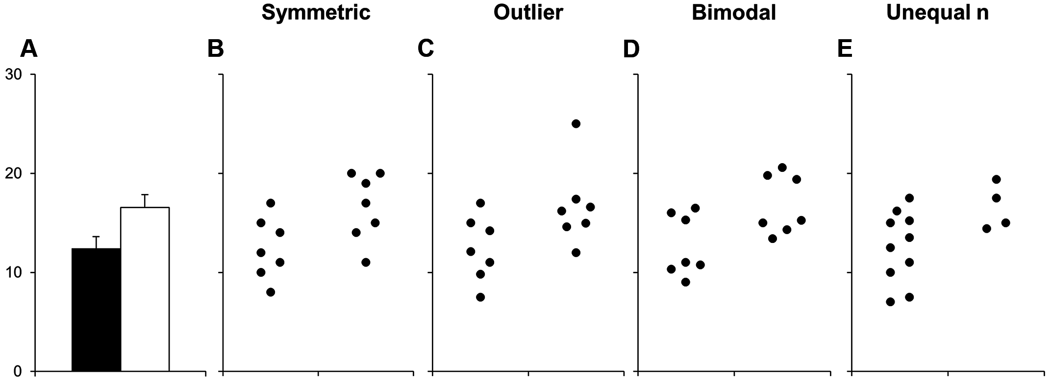
But remember, too, certain data visualization choices can obscure the data.
Distributions
Boxplots are one way to quickly highlight potential “outliers”. In the geom_boxplot() function it reads:
The upper whisker extends from the hinge to the largest value no further than 1.5 * IQR from the hinge (where IQR is the inter-quartile range, or distance between the first and third quartiles). The lower whisker extends from the hinge to the smallest value at most 1.5 * IQR of the hinge.
c_metrics |>
  pivot_longer(land_use_score_acre_yield_units:last_col()) |>
  ggplot(aes(y = crop, x = value)) +
  geom_boxplot(fill = "gray") +
  facet_wrap(vars(name), scales = "free_x", ncol = 2)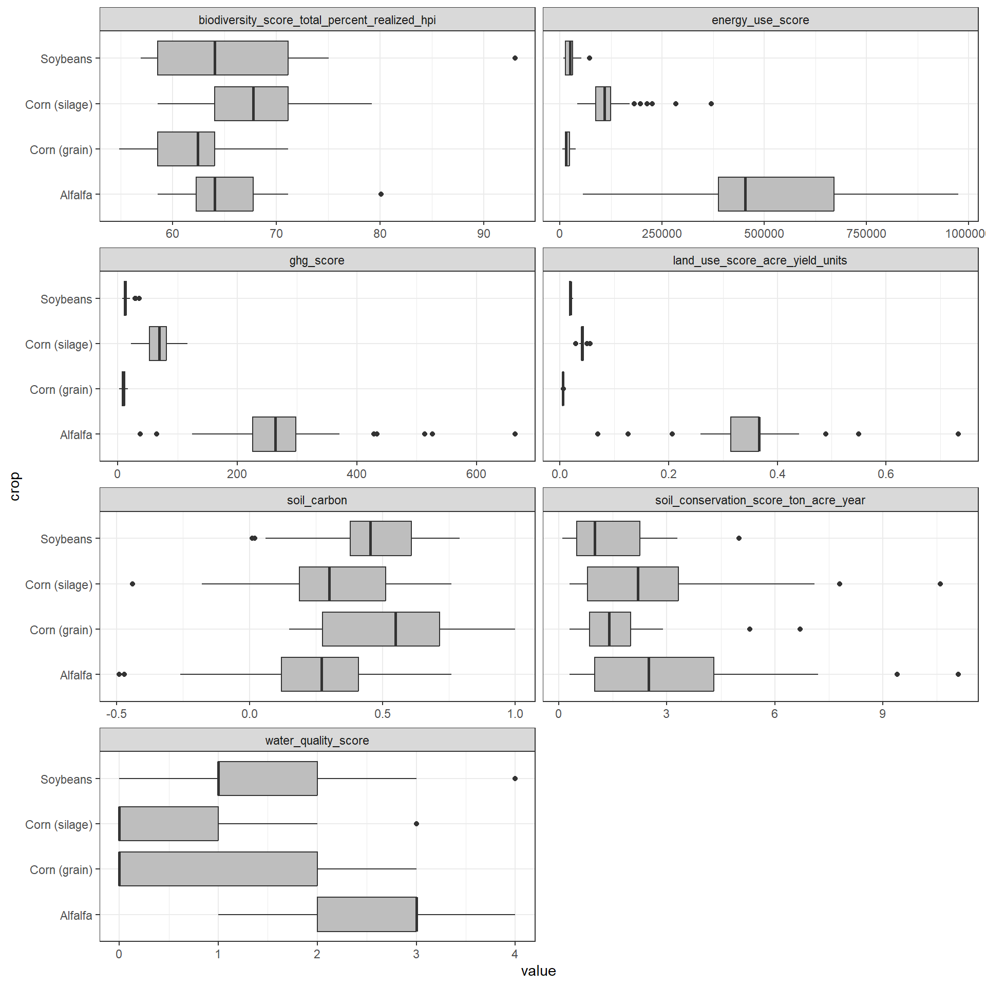
Try something a little more advanced such as the 5%, 50% (median), and 95% quantiles.
c_metrics |>
  pivot_longer(land_use_score_acre_yield_units:last_col()) |>
  ggplot(aes(y = crop, x = value,
             fill = factor(after_stat(quantile)))) +
  ggridges::stat_density_ridges(
    geom = "density_ridges_gradient",
    quantile_lines = TRUE,
    quantiles = c(0.025, 0.5, 0.975),
    scale = 1.2,
    rel_min_height = .01,
    jittered_points = FALSE, # make TRUE if you want
    point_shape = "|") +
  scale_color_manual(values = c("#13274FCC", "#A0A0A088")) +
  scale_fill_manual(
    name = "Probability",
    values = c("#13274FCC", "#A0A0A088", "#A0A0A088", "#CE1141CC"),
    labels = c("(0, 0.025]", "(0.025, 0.50)", "(0.025, 0.50)", "(0.975, 1]")) +
  facet_wrap(vars(name), scales = "free_x", ncol = 2)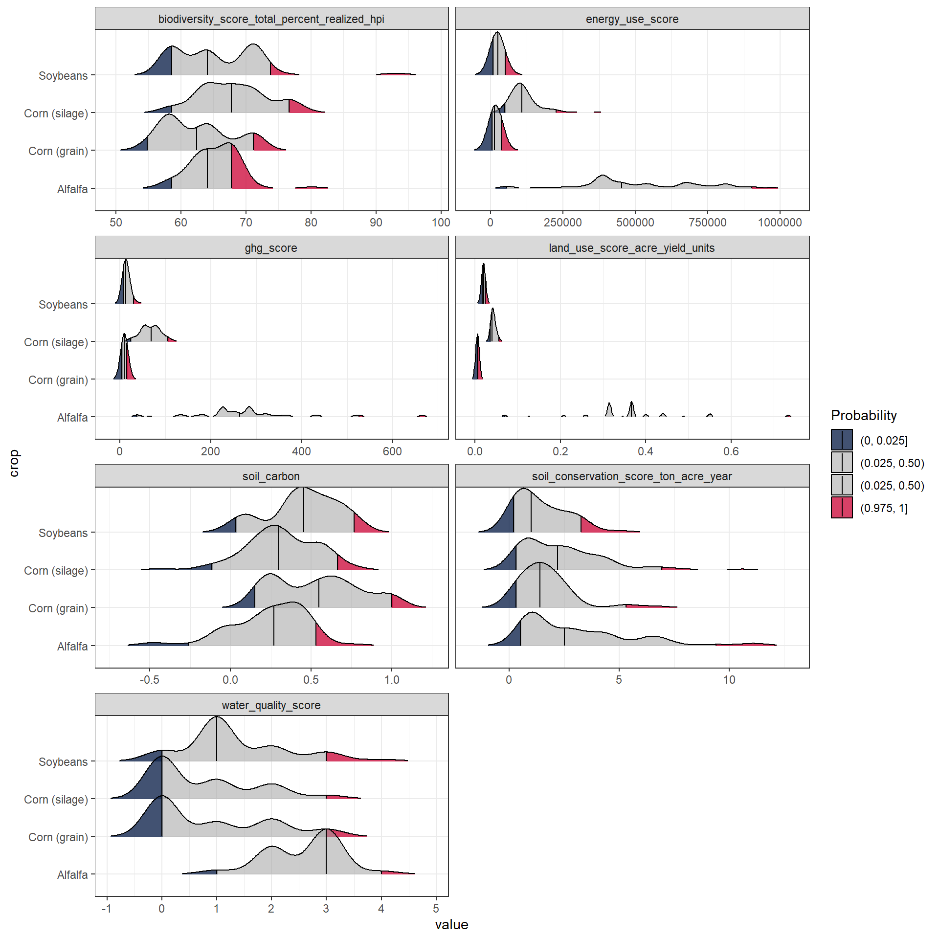
Yield is a key variable in many of the metrics. Therefore, let’s step back and see if we can spot any outliers in yield on an annual basis.
c_metrics |>
  ggplot(aes(x = crop_year, y = yield)) +
  geom_boxplot(aes(fill = crop_year)) +
  geom_jitter(width = 0.1, alpha = 0.3) +
  scale_fill_manual(values = c(gray, blue, orange)) +
  facet_wrap(vars(crop), scales = "free_y", ncol = 4)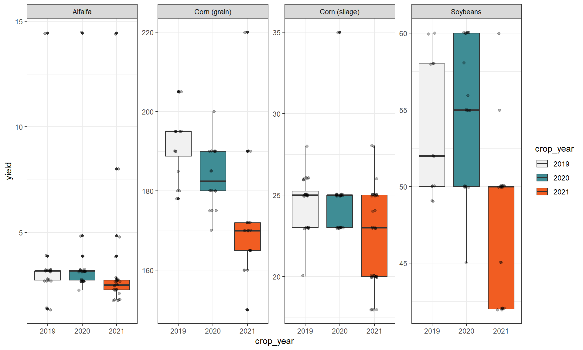
So, do you think the alfalfa yields around 14 ton/ac constitute an outlier?
Unless you have a clear reason to exclude a site (e.g., weather damage dropped yields > 90%), consider leaving it in.
Correlations
c_metrics |>
  filter(crop == "Alfalfa") |>
  select(where(is.numeric)) |>
  GGally::ggpairs()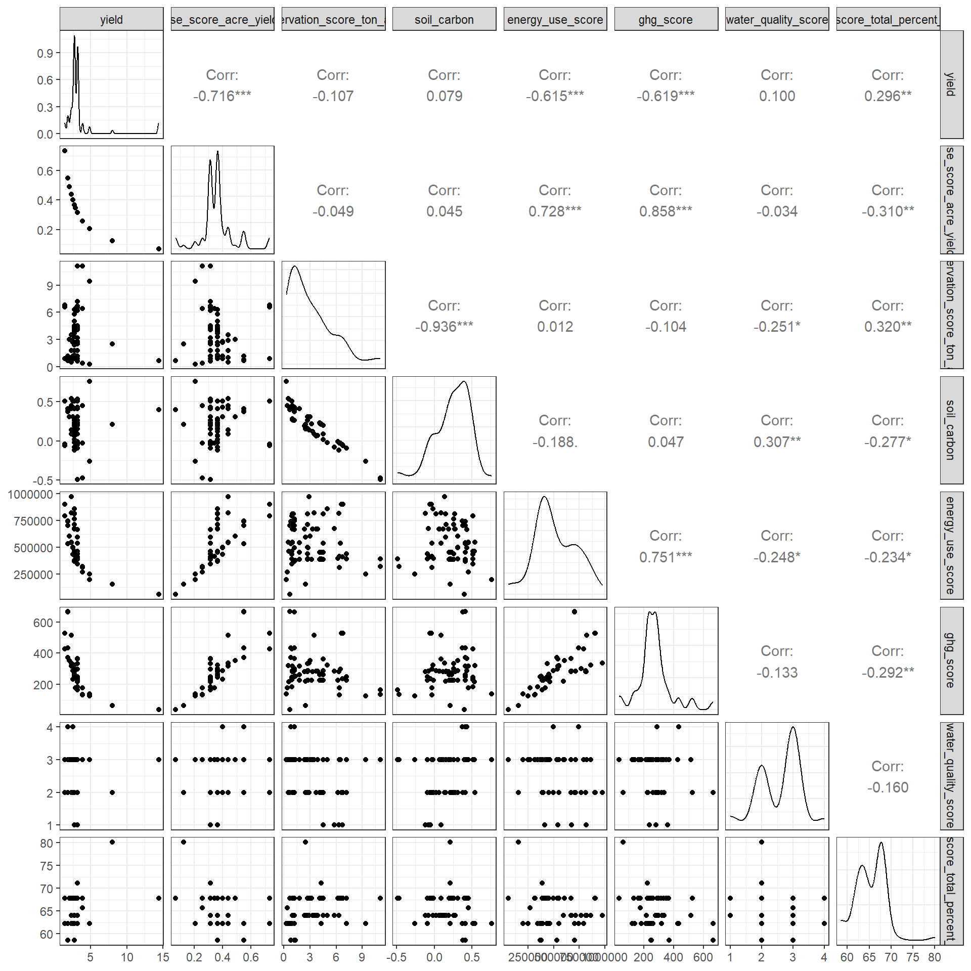
c_metrics |>
  ggplot(aes(x = yield, y = soil_conservation_score_ton_acre_year)) +
  geom_point() +
  facet_wrap(vars(crop), scales = "free") +
  geom_smooth(method = "lm")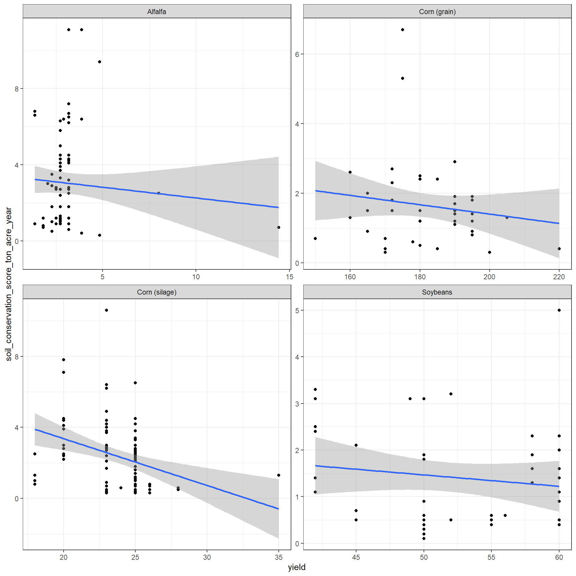
More involved Option
fit <- lm(ghg_score ~ yield,
          data = c_metrics |> filter(crop == "Alfalfa"))

olsrr::ols_plot_diagnostics(fit, print_plot = TRUE)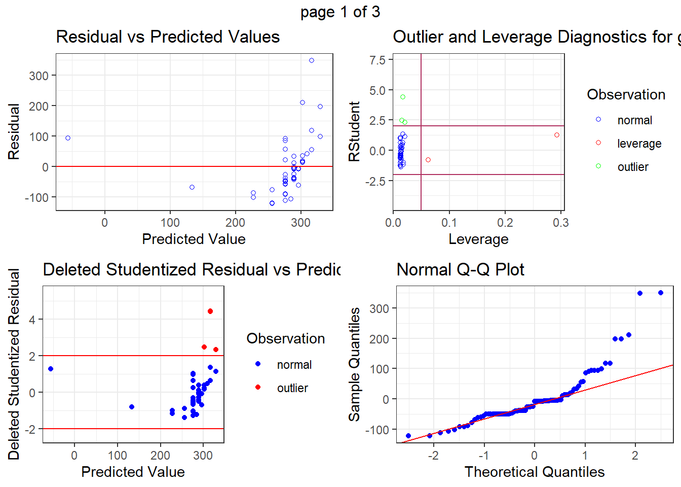
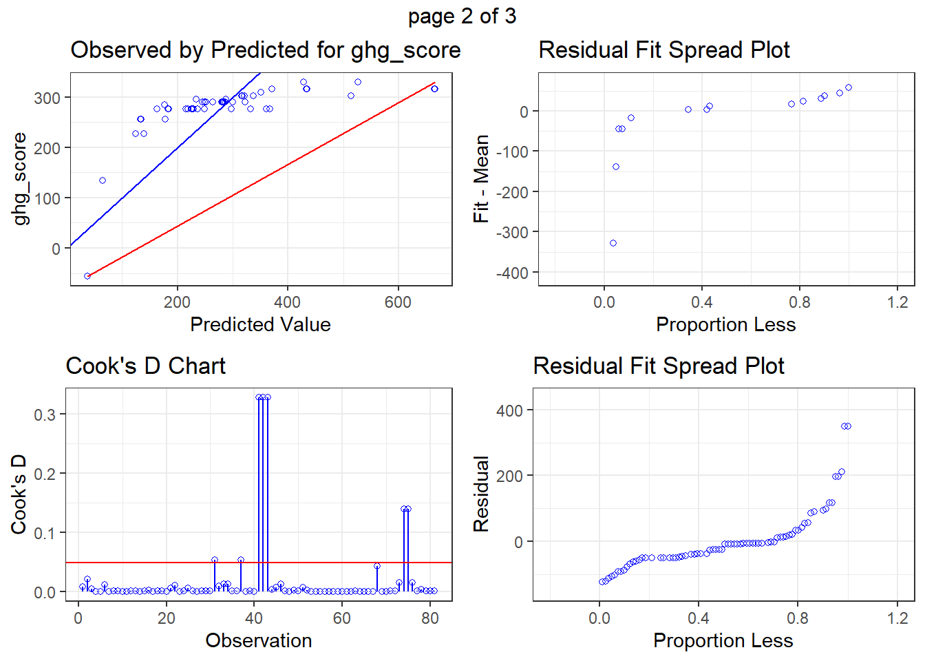
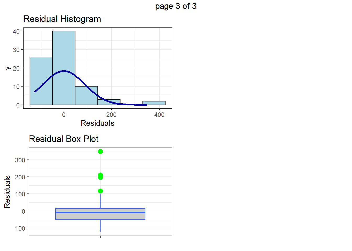
But again, unless you have a clear reason to exclude a site consider leaving it in.