10:00
Fieldprint Platform
2023 Data Analyst Training
Fieldprint Metrics
The cornerstone of Field to Market’s program lies in the sustainability metrics embedded within the Fieldprint Platform.
These metrics have been developed or adopted by Field to Market through the multi-stakeholder governance process over the past decade.
Energy Use ⛽
\(BTU/unit\)
All energy used in the production of one crop in one year, from pre-planting activities to the first point of sale.
Includes energy embodied in the seed, fertilizer, and chemicals applied to the fields. Factors from GREET and other sources.
GHG Emissions ☁️
\(lbs\ CO_2e/unit\)
Total GHG emissions from four main sources: energy use, nitrous oxide emissions from soils, methane emissions (from flooded fields), and residue burning.
Uses Energy Use, DayCent/DNDC metamodel
Soil Erosion ⛰️
\(\frac{ton}{ac}/year\)
Soil lost to erosion from water and wind as modeled through NRCS WEPP and WEPS using the crop rotation information.
Irrigation Water Use 🚿
\(ac\ in/unit\ increase\)
Account for the amount of water used to achieve an increase in crop yield.
Land Use 🏕️
\(ac/unit\)
Looks at productivity by accounting for how much land is used to produce a crop.
Biodiversity 🦆
\((0,100)\)
The Habitat Potential Index measures the capacity of a farm to support habitat for plants and animals. This could look at things like flooded rice fields that support migrating waterfowl, or edge of field areas that allow for wildlife to form habitat.
Soil Carbon 🌱
\((-1,1)\)
Utilizes the Soil Conditioning Index (SCI), a USDA NRCS tool, to analyze whether a field is gaining or losing carbon.
Water Quality 💧
\((0,4)\)
Uses the Stewardship Tool for Environmental Performance from NRCS to provide a detailed assessment of the risk of nutrient loss into local waterways through leaching and runoff, and shows how well practices are at mitigating that risk.
Break
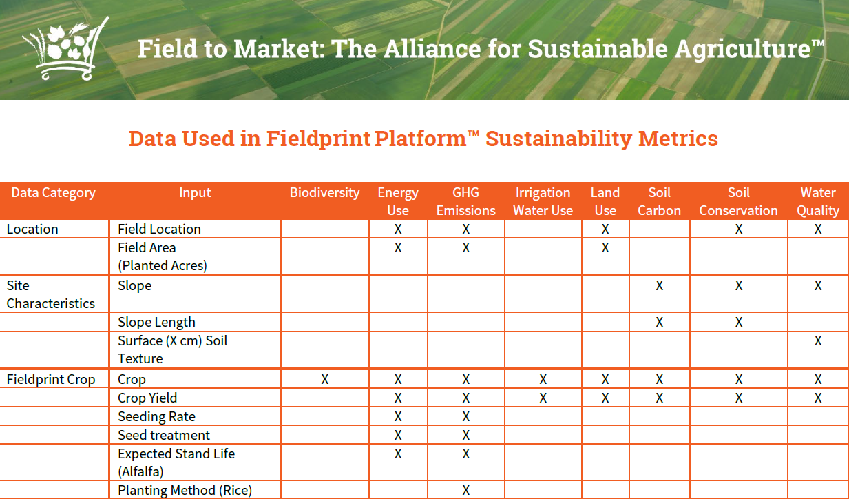
Put data in
Summary of inputs
QDMP
Qualified Data Management Partner
- Technology partners can embed our sustainability metrics in their own platforms through an API.
Demo
Get data out
Flow
- This is an iterative process as more data is added or data entries are fixed, changed, or corrected
Demo
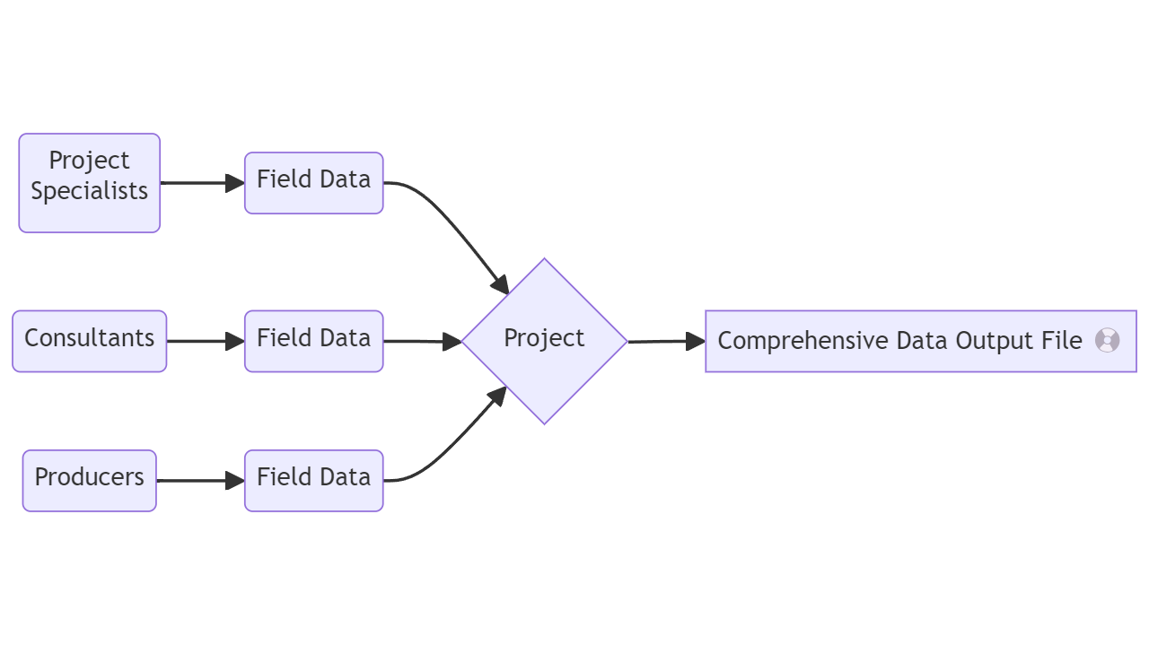
The CD 💿
The Comprehensive Data (CD) output file is a MS Excel file
really-long-name-with-metadata.xlsxRow = one grower, one field, one crop, one year
Columns = dynamic
- Number of columns varies according to the number of fertilizers and pesticide trips, and with the number of harvest operations for crops like alfalfa.
Hey, a data dictionary would be nice.
Exploratory Data Analysis
In obtaining your CD file, do you know:
What things to watch out for?
How to identify potential outliers?
How to check for data errors?
QA Tool Demo
Prep for analysis
fieldprintr
Still very early in development, the fieldprintr R package includes a dummy CD data frame called candyland and a wrapper function for importing CD *.xlsx files into R.

Import the “CD” file
# load libraries ----------------------------------------------------------
library(fieldprintr)
library(tidyverse)
library(skimr)
#library(scales)

theme_set(theme_bw())

orange <- "#f15d22"
blue <- "#3f8d95"
gray <- "#F1F1F1"

# read in comprehensive data file =============================================
# alternatively, use the readxl::read_xlsx() and janitor::clean_names() functions
raw_data <- fieldprintr::read_ftm_cd(
  "data/12-09-2022-1234_Comprehensive_Data_Candyland_Farms.xlsx")

# alternatively, use the built-in dataset
fieldprintr::candyland
Import the “CD” file
# A tibble: 300 × 422
   grower_id field_name      field_size_ac farm_serial_number tract_number
   <chr>     <chr>                   <dbl>              <dbl>        <dbl>
 1 432       10                       22.8                 NA        14634
 2 441       5a & 5b                  59.9                 NA        12254
 3 427       Bubblegum 1 & 2          41.6                 NA         5582
 4 427       Bubblegum 11             43.4                 NA        16327
 5 427       Bubblegum 13             20.7                 NA        16327
 6 427       Bubblegum 17N            14.5                 NA        16327
 7 427       Bubblegum 17S            11.6                 NA        16327
 8 427       Bubblegum 19E            19.5                 NA        16327
 9 427       Bubblegum 19W            41.1                 NA        16327
10 427       Bubblegum 23             23.1                 NA        16327
# ℹ 290 more rows
# ℹ 417 more variables: field_number <chr>, location <chr>, state <chr>,
#   field_geo_json <chr>, crop_year <chr>, crop <chr>, last_modified_on <dttm>,
#   metric_version <chr>, adjusted_yield <dbl>, adjusted_yield_units <chr>,
#   land_use_score_acre_yield_units <dbl>, total_soil_loss_year <dbl>,
#   soil_conservation_score_ton_acre_year <dbl>,
#   water_erosion_ton_acre_year <dbl>, wind_erosion_ton_acre_year <dbl>, …
First look at metric scores
Removed 18 irrigated fields to be analyzed separately.
# helper table for column filters
cols_scores <- read_csv(
  "data/CD-column-groupings.csv") |>
  # filter to just the fieldprint scores
  filter(group == "fieldprint_scores") |>
  pull(variable_clean)


c_metrics <-
  candyland |>
  filter(is_irrigated == "No") |>
  select(crop, crop_year,
         yield = adjusted_yield,
         all_of(cols_scores),
         # remove the character columns
         -energy_use_score_units, -ghg_score_units,
         # remove metrics that are not used (ex irrigation)
         -contains("irrigation"))
Note on Visualization
Without visualizations, summary values and statistical print outs can fall short. Our eyes are really useful for making sense of data.
Behold the importance of data visualization with [Datasaurus](https://cran.r-project.org/web/packages/datasauRus/vignettes/Datasaurus.html).
Note on Visualization
But remember, too, certain data visualization choices can obscure the data.
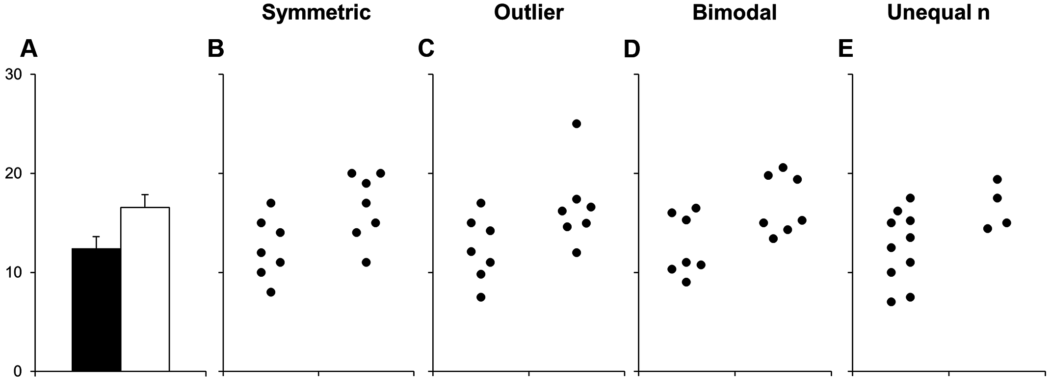
Weissgerber et al 2015. [Beyond Bar and Line Graphs: Time for a New Data Presentation Paradigm](https://doi.org/10.1371/journal.pbio.1002128)
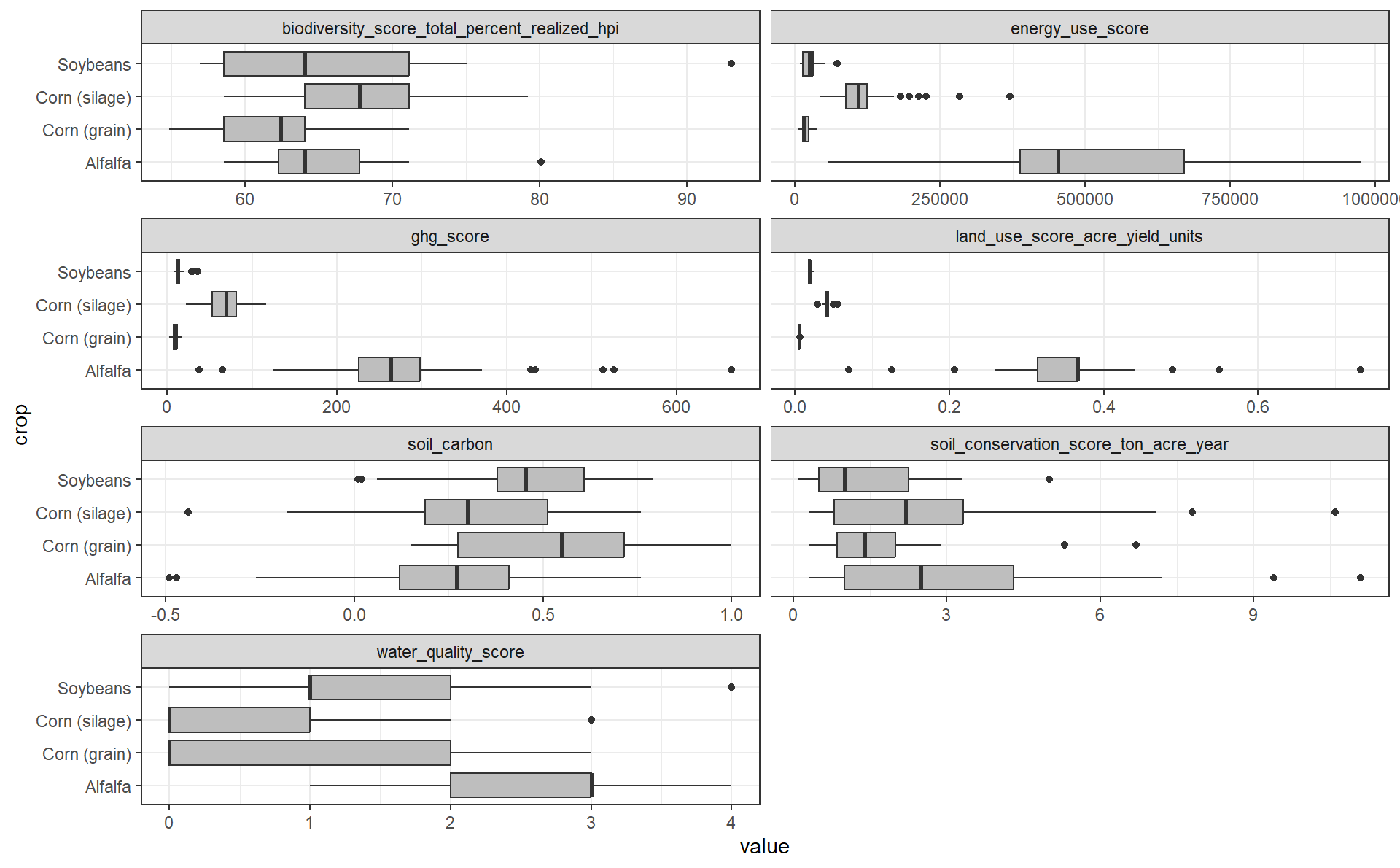
Distributions
Boxplots are one way to quickly highlight potential “outliers”. In the geom_boxplot() function it reads:
The upper whisker extends from the hinge to the largest value no further than 1.5 * IQR from the hinge (where IQR is the inter-quartile range, or distance between the first and third quartiles). The lower whisker extends from the hinge to the smallest value at most 1.5 * IQR of the hinge.
Boxplot
Boxplot
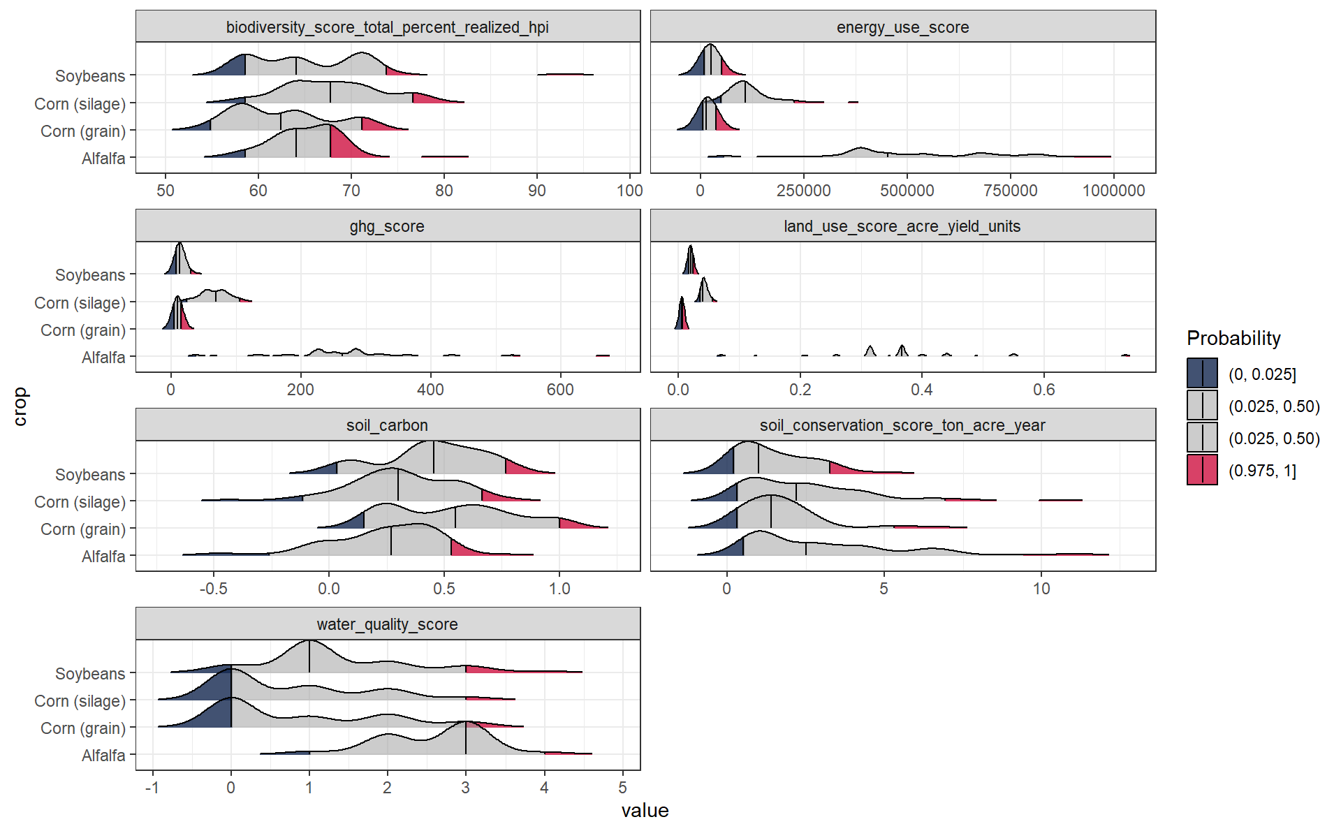
Distributions with 95% interval
Try something a little more advanced such as the 5%, 50% (median), and 95% quantiles.
c_metrics |>
  pivot_longer(land_use_score_acre_yield_units:last_col()) |>
  ggplot(aes(y = crop, x = value,
             fill = factor(after_stat(quantile)))) +
  ggridges::stat_density_ridges(
    geom = "density_ridges_gradient",
    quantile_lines = TRUE,
    quantiles = c(0.025, 0.5, 0.975),
    scale = 1.2,
    rel_min_height = .01,
    jittered_points = FALSE, # make TRUE if you want
    point_shape = "|") +
  scale_color_manual(values = c("#13274FCC", "#A0A0A088")) +
  scale_fill_manual(
    name = "Probability",
    values = c("#13274FCC", "#A0A0A088", "#A0A0A088", "#CE1141CC"),
    labels = c("(0, 0.025]", "(0.025, 0.50)", "(0.025, 0.50)", "(0.975, 1]")) +
  facet_wrap(vars(name), scales = "free_x", ncol = 2)
Distributions with 95% interval
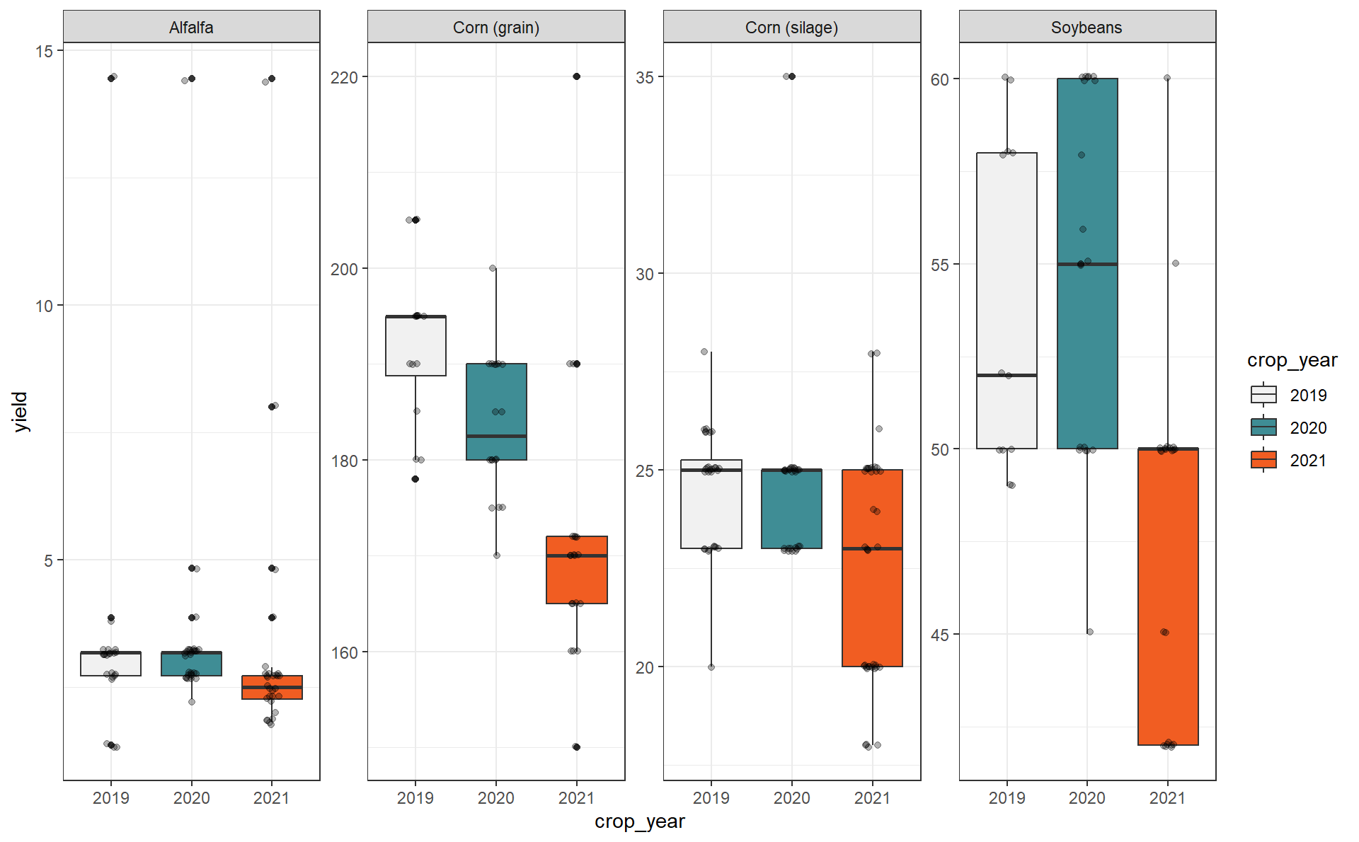
Step back and check for yield
Yield is a key variable in many of the metrics. Therefore, let’s step back and see if we can spot any outliers in yield on an annual basis.
Step back and check for yield
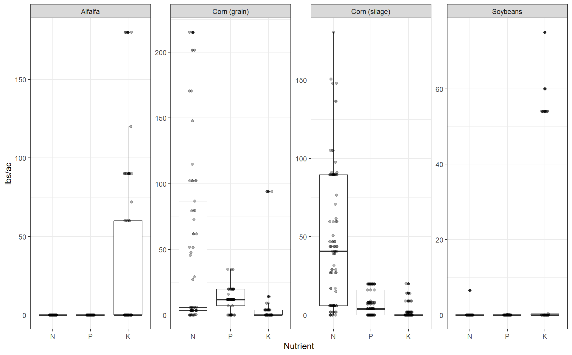
Checking for errors
The Fieldprint Platform has boundaries implemented for all nutrients for an individual operation. It is possible to enter excessive amounts of fertilizer when operations are aggregated.
Some agronomic knowledge is needed to judge if fertilizer and manure amounts are appropriate for the regions included in a project.
Fertilizer
candyland |>
  rename(N = total_n_lb_acre_for_all_trips,
         P = total_p2o5_lb_acre_for_all_trips,
         K = total_k2o_lb_acre_for_all_trips) |>
  pivot_longer(cols = c(N, P, K),
               names_to = "Nutrient",
               values_to = "Rate") |>
  ggplot(aes(x = fct_relevel(Nutrient, "N", "P", "K"), y = Rate)) +
  geom_boxplot() +
  geom_jitter(width = 0.1, alpha = 0.3) +
  scale_fill_manual(values = c(gray, blue, orange, "white")) +
  facet_wrap(vars(crop), scales = "free_y", ncol = 4) +
  labs(x = "Nutrient",
       y = "lbs/ac") +
  guides(fill = "none")
Fertilizer
Protectants
candyland |>
  rename(Herbicide = total_herbicides_for_all_trips,
         Insecticide = total_insecticides_for_all_trips,
         Fungicide = total_fungicides_for_all_trips,
         GrowthRegulator = total_growth_regulators_for_all_trips,
         Fumigant = total_fumigant_for_all_trips) |>
  pivot_longer(cols = c(Herbicide,
                        Insecticide,
                        Fungicide,
                        GrowthRegulator,
                        Fumigant),
               names_to = "Protectants",
               values_to = "applications") |>
  ggplot(aes(x = Protectants, y = applications, color = crop)) +
  geom_jitter(height = 0.01, width = 0.2, alpha = 0.1) +
  scale_color_manual(values = c("black", blue, orange, "#002255")) +
  facet_wrap(vars(crop), scales = "free_y", ncol = 2) +
  labs(x = "",
       y = "Number of Applications") +
  guides(fill = "none")
Protectants
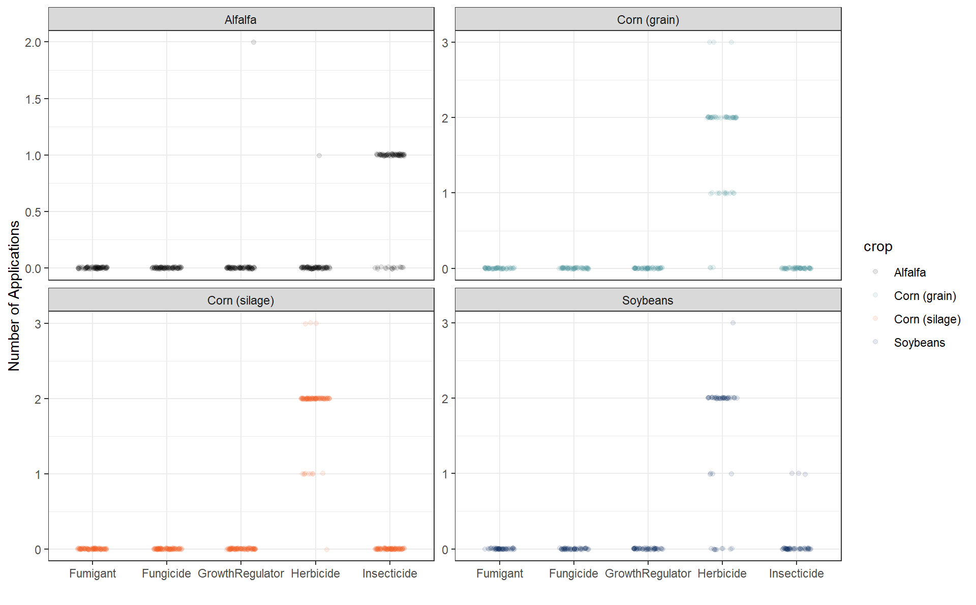
Protectants
Does herbicide usage seem too high?
Is there high incidence of herbicide-resistant weeds?
Do we need to collaborate with an agronomist/weed specialist?
May be opportunities for improvement if we understand why some producers are applying more or less
Homework
Office hours
Session One