Benchmarks and Beyond
2023 Data Analyst Training
Project Benchmarks
The primary purpose of comparisons and benchmarks is to provide context to growers to understand how their performance relates to that of their peers.
What is your scope?
- If the project covers a large area (e.g., multiple states) you may wish to create more than one set of project benchmarks distinct to a subset of your project population.
- Benchmarks should also be calculated separately for irrigated and non-irrigated production, if both are present in a Project.
Demo: Averaging metric scores

Can I just report the mean values?
No. The simple arithmetic means listed above are based on dividing the sum of the metric values by the number of fields. In this perspective, a 1-acre field has the same environmental impact as a 100-acre field.
Consider this scenario
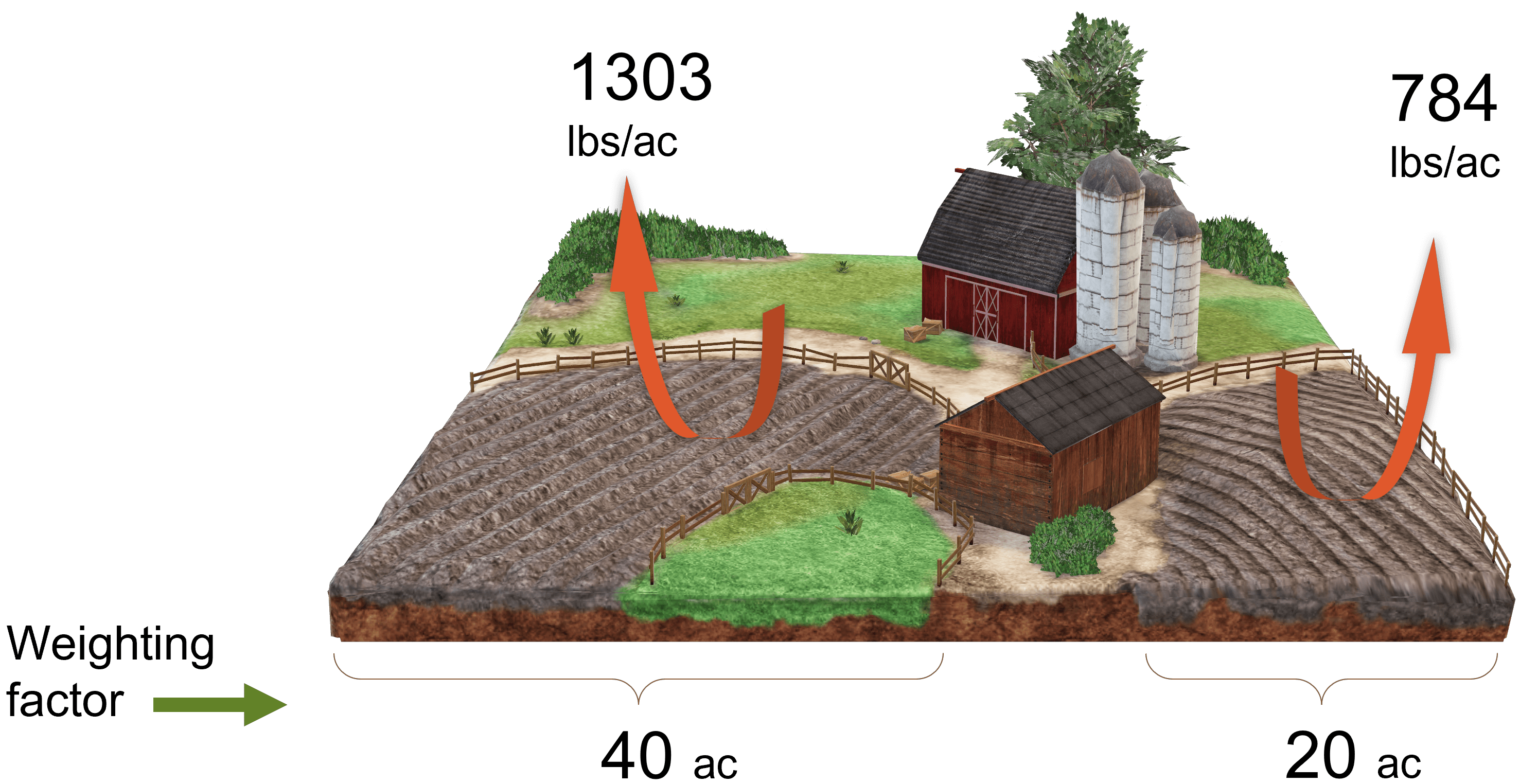
How should the average CO2 emission be reported?
Simple Mean
[1] "1043.5 lbs CO2/ac"Weighted Means
The weighted mean is the sum of the metric totals across the project fields divided by the sum of the weighting factor across the same fields.
We suggest two weighting factors: field area and field production. Doing so means that the largest fields and/or most productive fields carry the most weight in the final average.
Weighted Means
[1] 1130[1] "1130 lbs CO2/ac"Consider this scenario
In the above example, the average emission is closer to 1130 lbs CO2e/ac, not 1043, because the majority of the land is responsible for the majority of emissions.
Caution
The weighting factor must correspond to the units of the metric score. In other words:
use area-weighted means for a metric score expressed on per acre basis
use production-weighted means for a metric score expressed on a production basis
Interpretation
“How many lbs of CO2e were emitted to produce the average [unit] of [crop]?”
“How many lbs of CO2e were emitted on the average acre?”
“How many lbs of CO2e were emitted on the acre that produced the average [unit] of [crop]?”
“How many lbs of CO2e were emitted to produce a [unit] of [crop] on the average acre?”
Demo: Averaging metric scores in Excel
Weighted means in R
As an R function, this is what a project “benchmark” calculation could look like:
# Area-weighted benchmark for metric with units on an area basis
benchmark_area <- function(data, metric) {
  data |>
  group_by(crop, crop_year) |>
  summarize(
    total_area   = sum(field_size_ac),
    total_metric = sum({{metric}} * field_size_ac),
    simple_mean  = mean({{metric}}),
    wt_mean      = total_metric / total_area,
    weight_factor = "area") |>
  ungroup()
}
Weighted means in R
# Production-weighted benchmark for metric with units on an area basis
benchmark_prod <- function(data, metric) {
data |>
group_by(crop, crop_year) |>
summarize(
total_prod = sum(production),
total_metric = sum({{metric}} * production),
simple_mean = mean({{metric}}),
wt_mean = total_metric / total_prod,
weight_factor = "production") |>
ungroup()
}
c_ghg <-
candyland |>
filter(is_irrigated == "No") |>
select(grower_id, field_name, crop, crop_year,
ghg_score, ghg_score_units, # for production weighting
ghg_per_acre_lbs_co2e_acre, # for area weighting
field_size_ac, adjusted_yield) |>
mutate(production = adjusted_yield * field_size_ac) # for production weighting
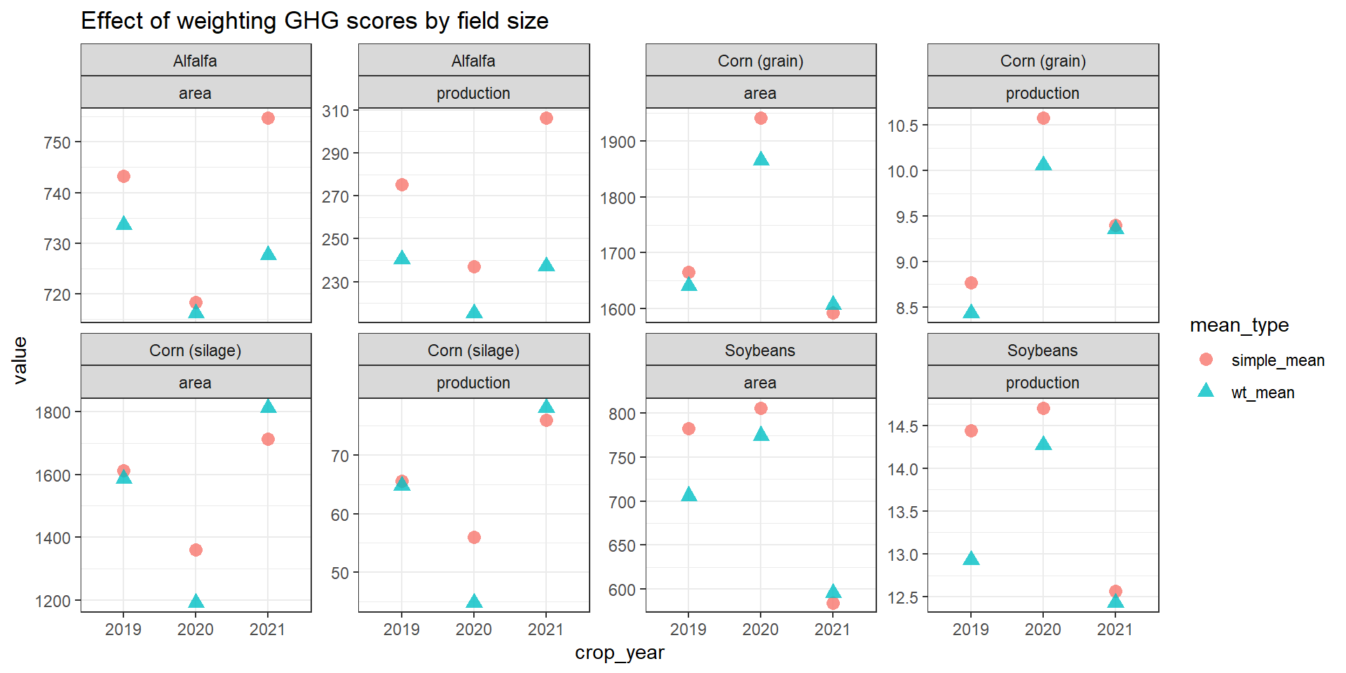
#--notice the units of ghg_score are per unit yield and depend on the crop Visualize the difference between mean and weighted mean
c_ghg_wt <- bind_rows(
  benchmark_prod(c_ghg, ghg_score),
  benchmark_area(c_ghg, ghg_per_acre_lbs_co2e_acre))

c_ghg_wt |>
  pivot_longer(simple_mean:wt_mean,
               names_to = "mean_type") |>
  ggplot(aes(crop_year, value)) +
  geom_point(aes(shape = mean_type,
                 color = mean_type),
             size = 3,
             alpha = 0.8) +
  facet_wrap(vars(crop, weight_factor), scales = "free_y", ncol = 4) +
  labs(title = "Effect of weighting GHG scores by field size")
Visualize the difference between mean and weighted mean
Break
10:00
Efficiency Metrics

Efficiency Metrics
Over time, will a production system ONLY reduce inputs while maintaining outputs?
Or will it instead increase outputs justified by improved efficiency?
Importance of reporting total impacts
How much irrigation water was used?
c_water <- candyland |>
  filter(is_irrigated == "Yes") |>
  mutate(
    groundwater = replace_na(groundwater_irrigation_water_applied_acre_inch_acre, 0),
    surface = replace_na(surface_water_irrigation_water_applied_acre_inch_acre, 0),
    total_irrigation = (groundwater + surface) * field_size_ac)

c_water |>
  ggplot(aes(crop, total_irrigation, color = crop_year)) +
  geom_jitter(width = 0.1)
How much irrigation water was used?
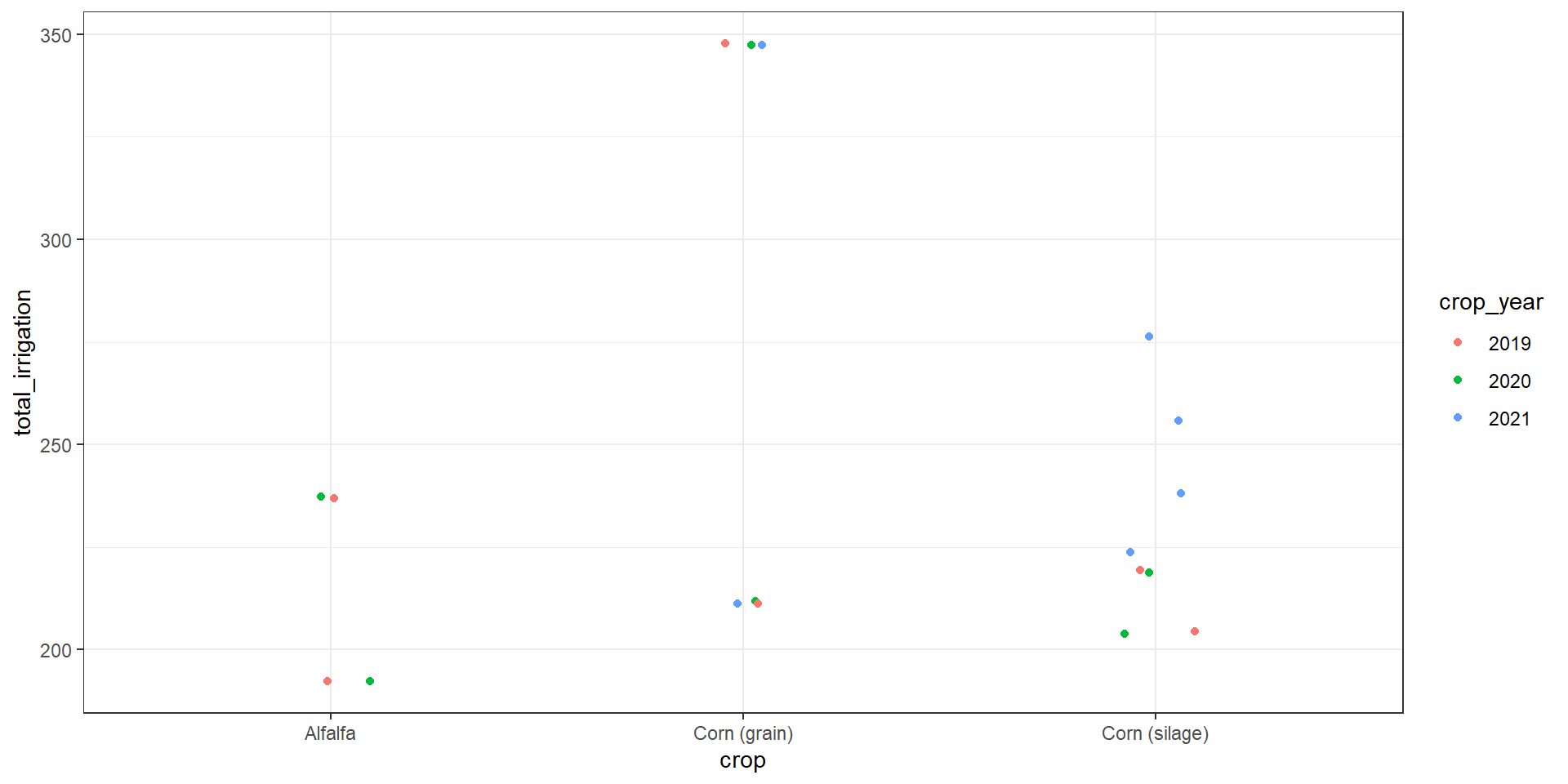
How much irrigation water was used?
# A tibble: 3 × 3
  crop          avg_irrigation     n
  <chr>                  <dbl> <int>
1 Alfalfa                 214.     4
2 Corn (grain)            280.     6
3 Corn (silage)           230      8
How does that water use compare to state averages?
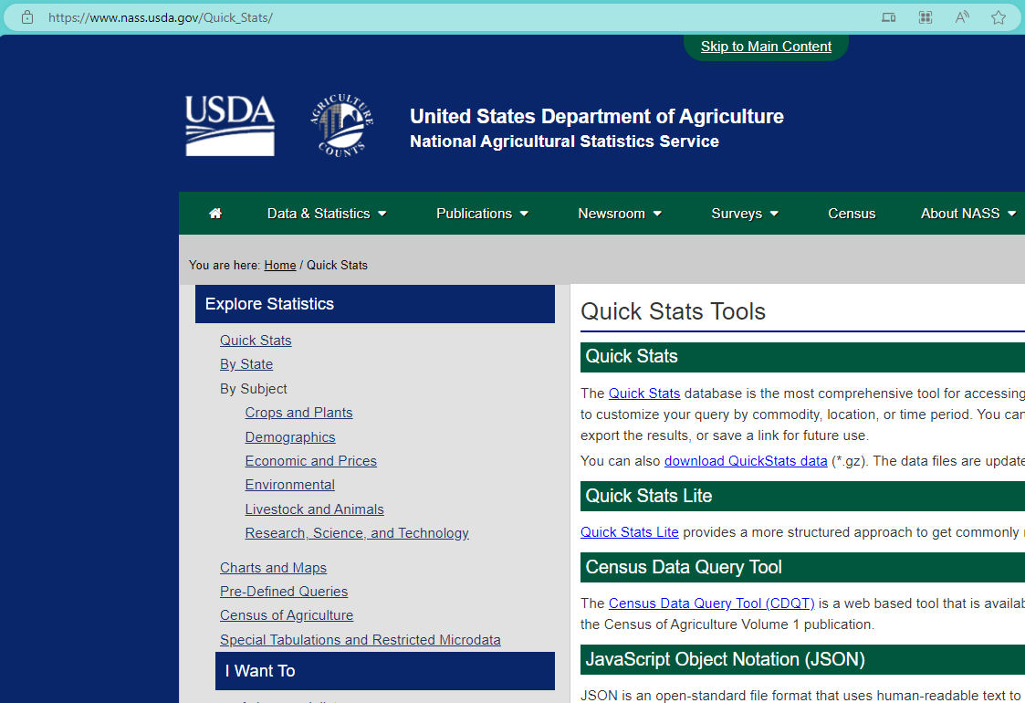
Using NASS statistics
NASS query by desktop
NASS query by R
# Function for getting NASS data
get_nass_water <- function(years,
                           #source = "SURVEY",
                           crops = NULL){

    params_list <- list(
        year = years,
        commodity_desc = crops,
        #source_desc = source,
        sector_desc = "CROPS",
        group_desc = c("FIELD CROPS"),
        statisticcat_desc = "WATER APPLIED",
        reference_period_desc = "YEAR",
        agg_level_desc = c("STATE")
    )

    n_records <- nassqs_record_count(params_list)$count
    assertthat::assert_that(n_records < 50000)

    output_df <- nassqs(params_list) |>
        as_tibble()

    return(output_df)

}
  |
  |                                                                      |   0%
  |
  |======================================================================| 100%

  |
  |                                                                      |   0%
  |
  |===                                                                   |   4%
  |
  |======                                                                |   8%
  |
  |=========                                                             |  12%
  |
  |============                                                          |  16%
  |
  |==============                                                        |  21%
  |
  |=================                                                     |  25%
  |
  |====================                                                  |  29%
  |
  |=======================                                               |  33%
  |
  |==========================                                            |  37%
  |
  |=============================                                         |  41%
  |
  |===================================                                   |  50%
  |
  |======================================                                |  54%
  |
  |=========================================                             |  58%
  |
  |============================================                          |  62%
  |
  |==============================================                        |  66%
  |
  |=================================================                     |  70%
  |
  |====================================================                  |  75%
  |
  |=======================================================               |  79%
  |
  |==========================================================            |  83%
  |
  |=============================================================         |  87%
  |
  |================================================================      |  91%
  |
  |===================================================================   |  95%
  |
  |======================================================================| 100%
# A tibble: 13 × 6
source_desc year commodity_desc class_desc util_practice_desc n
<chr> <chr> <chr> <chr> <chr> <int>
1 CENSUS 2018 BEANS DRY EDIBLE, INCL C… ALL UTILIZATION P… 57
2 CENSUS 2018 CORN ALL CLASSES GRAIN 112
3 CENSUS 2018 CORN ALL CLASSES SILAGE 87
4 CENSUS 2018 COTTON ALL CLASSES ALL UTILIZATION P… 51
5 CENSUS 2018 HAY & HAYLAGE (EXCL ALFALFA) ALL UTILIZATION P… 86
6 CENSUS 2018 HAY & HAYLAGE ALFALFA ALL UTILIZATION P… 88
7 CENSUS 2018 PASTURELAND ALL CLASSES ALL UTILIZATION P… 108
8 CENSUS 2018 PEANUTS ALL CLASSES ALL UTILIZATION P… 28
9 CENSUS 2018 RICE ALL CLASSES ALL UTILIZATION P… 21
10 CENSUS 2018 SMALL GRAINS OTHER ALL UTILIZATION P… 68
11 CENSUS 2018 SORGHUM ALL CLASSES GRAIN 35
12 CENSUS 2018 SOYBEANS ALL CLASSES ALL UTILIZATION P… 82
13 CENSUS 2018 WHEAT ALL CLASSES ALL UTILIZATION P… 87NASS query by R
raw_irrigation |>
  filter(commodity_desc %in% c("CORN", "HAY & HAYLAGE", "SOYBEANS"),
         class_desc != c("(EXCL ALFALFA)"),
         state_name %in% c("WISCONSIN", "MISSOURI", "ILLINOIS")) |>
  group_by(state_name,
           commodity_desc,
           class_desc,
           util_practice_desc,
           domaincat_desc) |>
  summarize(water_applied = mean(Value * 12, na.rm = TRUE)) |>
  ungroup() |>
  select(-class_desc) |>
  print(n = 30)
NASS query by R
# A tibble: 22 × 5
   state_name commodity_desc util_practice_desc     domaincat_desc water_applied
   <chr>      <chr>          <chr>                  <chr>                  <dbl>
 1 ILLINOIS   CORN           GRAIN                  IRRIGATION ME…           7.2
 2 ILLINOIS   CORN           GRAIN                  NOT SPECIFIED            7.2
 3 ILLINOIS   SOYBEANS       ALL UTILIZATION PRACT… IRRIGATION ME…           6
 4 ILLINOIS   SOYBEANS       ALL UTILIZATION PRACT… NOT SPECIFIED            6
 5 MISSOURI   CORN           GRAIN                  IRRIGATION ME…          12
 6 MISSOURI   CORN           GRAIN                  IRRIGATION ME…           7.2
 7 MISSOURI   CORN           GRAIN                  NOT SPECIFIED            8.4
 8 MISSOURI   CORN           SILAGE                 IRRIGATION ME…           3.6
 9 MISSOURI   CORN           SILAGE                 NOT SPECIFIED            3.6
10 MISSOURI   HAY & HAYLAGE  ALL UTILIZATION PRACT… IRRIGATION ME…           3.6
11 MISSOURI   HAY & HAYLAGE  ALL UTILIZATION PRACT… NOT SPECIFIED            3.6
12 MISSOURI   SOYBEANS       ALL UTILIZATION PRACT… IRRIGATION ME…           8.4
13 MISSOURI   SOYBEANS       ALL UTILIZATION PRACT… IRRIGATION ME…           7.2
14 MISSOURI   SOYBEANS       ALL UTILIZATION PRACT… NOT SPECIFIED            8.4
15 WISCONSIN  CORN           GRAIN                  IRRIGATION ME…           6
16 WISCONSIN  CORN           GRAIN                  NOT SPECIFIED            6
17 WISCONSIN  CORN           SILAGE                 IRRIGATION ME…           4.8
18 WISCONSIN  CORN           SILAGE                 NOT SPECIFIED            4.8
19 WISCONSIN  HAY & HAYLAGE  ALL UTILIZATION PRACT… IRRIGATION ME…           4.8
20 WISCONSIN  HAY & HAYLAGE  ALL UTILIZATION PRACT… NOT SPECIFIED            4.8
21 WISCONSIN  SOYBEANS       ALL UTILIZATION PRACT… IRRIGATION ME…           4.8
22 WISCONSIN  SOYBEANS       ALL UTILIZATION PRACT… NOT SPECIFIED            4.8
What percent of acres received a cover crop?
Further Considerations
Detrending Fieldprint Platform Yield-based Metrics Using NASS Data
How different would the final scores be if the answers given in the Calculator were changed?
In other words, “How sensitive is each metric to my inputs?”
This interactive website for sensitivity analysis was built by Eric Coronel
Session Two